We recently estimated the risk of opioid use disorder and opioid overdose that is due to having a chronic pain condition or a physical disability (total effects).
Having a chronic pain condition (without disability) more than doubled the risk (3.6% developed OUD in 18 mo).
Having a physical disability (without chronic pain) increased risk by more than 1.6 times (2.9% developed OUD).
To what extent are these total risks explained by the pain management treatments that result from these conditions? Which treatments are more risky? Which are less risky?
We can to use mediation analysis to explore the pain management mechanisms contributing to these risks.
Key questions:
To what extent does the effect of having a disability or chronic pain condition at the time of Medicaid enrollment on subsequent OUD risk operate through pain management strategies? Considered as a bundle? And one-by-one? (Rudolph et al. 2025)
Rudolph, Kara E, Shodai Inose, Nicholas T Williams, Katherine L Hoffman, Sarah E Forrest, Rachael K Ross, Floriana Milazzo, et al. 2025. “Mediation of Chronic Pain and Disability on Opioid Use Disorder Risk by Pain Management Practices Among Adult Medicaid Patients, 2016-2019.”American Journal of Epidemiology, kwaf093.
1.2 What is causal mediation analysis?
Statistical mediation analyses assess associations between the variables. They can help you establish, for example, if the association between treatment and outcome can be mostly explained by an association between treatment and mediator
Causal mediation analyses, on the other hand, seek to assess causal relations. For example, they help you establish whether treatment causes the outcome because it causes the mediator. To do this, causal mediation seek to understand how the paths behave under circumstances different from the observed circumstances (e.g., interventions)
1.2.1 Why are the causal methods that we will discuss today important?
Assume you are interested in the effect of treatment assignment \(A\) (e.g., chronic pain condition vs. neither chronic pain nor physical disability) on an outcome \(Y\) (risk of OUD) through mediators \(M\) (e.g., opioid prescriptions, co-prescriptions, anti-depressants and anti-inflammatories, physical therapy)
We have pre-treatment confounders \(W\)
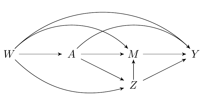
When considering particular pain management treatments, there are intermediate confounders, \(Z\), of the \(M \rightarrow Y\) relationship that are affected by chronic pain: other co-occurring or upstream pain management treatments
We could fit the following models: \[\begin{align}
\E(M \mid A=a, W=w, Z=z) & = \gamma_0 + \gamma_1 a + \gamma_2 w + \gamma_3 z \\
\E(Y \mid M=m, A=a, W=w, Z=z) & = \beta_0 + \beta_1 m + \beta_2 a + \beta_3 w + \beta_4 z
\end{align}\]
The product \(\gamma_1 \beta_1\) has been proposed as a measure of the effect of \(A\) on \(Y\) through \(M\)
Causal interpretation problems with this method: We will see that this parameter cannot be interpreted as a causal effect
1.2.2R Example:
Assume we have a pre-treatment confounder of \(Y\) and \(M\), denote it with \(W\)
For simplicity, assume \(A\) is randomized
We’ll generate a really large sample from a data generating mechanism so that we are not concerned with sampling errors
Note that the indirect effect (i.e., the effect through \(M\)) in this example is nonzero (there is a pathway \(A \rightarrow Z \rightarrow M \rightarrow Y\))
Let’s see what the product of coefficients method would say:
Among other things, in this workshop:
We will provide some understanding for why the above method fails in this example
We will study estimators that are robust to misspecification in the above models
1.3 Causal mediation models
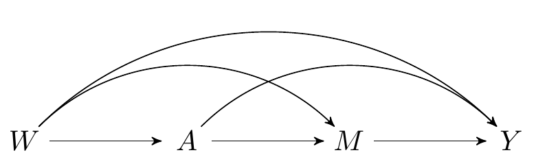
In this workshop we will use directed acyclic graphs. We will focus on the two types of graph:
Directed acyclic graph under intermediate confounders of the mediator-outcome relation affected by treatment
The above graphs can be interpreted as a non-parametric structural equation model (NPSEM), also known as structural causal model (SCM):
\[\begin{align}
W & = f_W(U_W) \nonumber \\
A & = f_A(W, U_A) \nonumber \\
Z & = f_Z(W, A, U_Z) \nonumber \\
M & = f_M(W, A, Z, U_M) \nonumber \\
Y & = f_Y(W, A, Z, M, U_Y)
\end{align}\]
Here \(U=(U_W, U_A, U_Z, U_M, U_Y)\) is a vector of all unmeasured exogenous factors affecting the system
The functions \(f\) are assumed fixed but unknown
We posit this model as a system of equations that nature uses to generate the data
Therefore we leave the functions \(f\) unspecified (i.e., we do not know the true nature mechanisms)
Sometimes we know something: e.g., if \(A\) is randomized we know \(A=f_A(U_A)\) where \(U_A\) is the flip of a coin (i.e., independent of everything).
1.4 Counterfactuals
Recall that we are interested in assessing how the pathways would behave under circumstances different from the observed circumstances
We operationalize this idea using counterfactual random variables
Counterfactuals are hypothetical random variables that would have been observed in an alternative world where something had happened, possibly contrary to fact
1.4.1 We will use the following counterfactual variables:
\(Y_a\) is a counterfactual variable in a hypothetical world where \(\P(A=a)=1\) for some value \(a\)
\(Y_{a,m}\) is the counterfactual outcome in a world where \(\P(A=a,M=m)=1\)
\(M_a\) is the counterfactual variable representing the mediator in a world where \(\P(A=a)=1\).
1.4.2 How are counterfactuals defined?
In the NPSEM framework, counterfactuals are quantities derived from the model.
Once you define a change to the causal system, that change needs to be propagated downstream.
Example: modifying the system to make everyone receive XR-NTX yields counterfactual adherence, mediators, and outcomes.
Take as example the DAG in Figure 1.2: \[\begin{align}
A &= a \nonumber \\
Z_a &= f_Z(W, a, U_Z) \nonumber \\
M_a &= f_M(W, a, Z_a, U_M) \nonumber \\
Y_a &= f_Y(W, a, Z_a, M_a, U_Y)
\end{align}\]
We will also be interested in joint changes to the system: \[\begin{align}
A &= a \nonumber \\
Z_a &= f_Z(W, a, U_Z) \nonumber \\
M &= m \nonumber \\
Y_{a,m} &= f_Y(W, a, Z_a, m, U_Y)
\end{align}\]
And, perhaps more importantly, we will use nested counterfactuals
For example, if \(A\) is binary, you can think of the following counterfactual \[\begin{align}
A &= 1 \nonumber \\
Z_1 &= f_Z(W, 1, U_Z) \nonumber \\
M &= M_0 \nonumber \\
Y_{1, M_0} &= f_Y(W, 1, Z_1, M_0, U_Y)
\end{align}\]
\(Y_{1, M_0}\) is interpreted as the outcome for an individual in a hypothetical world where treatment was given but the mediator was held at the value it would have taken under no treatment.
Causal mediation effects are often defined in terms of the distribution of these nested counterfactuals.
That is, causal effects give you information about what would have happened in some hypothetical world where the mediator and treatment mechanisms changed.
Source Code
# Causal mediation analysis intro {#mediation}```{r}#| label: load-renv#| echo: false#| message: falserenv::autoload()library(here)```## Motivating study- We recently estimated the risk of opioid use disorder and opioid overdose that is due to having a chronic pain condition or a physical disability (total effects). - Having a chronic pain condition (without disability) more than doubled the risk (3.6% developed OUD in 18 mo). - Having a physical disability (without chronic pain) increased risk by more than 1.6 times (2.9% developed OUD).- To what extent are these total risks explained by the pain management treatments that result from these conditions? Which treatments are more risky? Which are less risky?- We can to use mediation analysis to explore the pain management mechanisms contributing to these risks.- Key questions: - To what extent does the effect of having a disability or chronic pain condition at the time of Medicaid enrollment on subsequent OUD risk operate through pain management strategies? Considered as a bundle? And one-by-one? [@rudolph2025mediation]{width="80%"}{width="80%"}## What is causal mediation analysis?- Statistical mediation analyses assess associations between the variables. They can help you establish, for example, if the *association* between treatment and outcome can be mostly explained by an *association* between treatment and mediator- Causal mediation analyses, on the other hand, seek to assess causal relations. For example, they help you establish whether treatment *causes* the outcome because it *causes* the mediator. To do this, causal mediation seek to understand how the paths behave under circumstances different from the observed circumstances (e.g., interventions)<!--- Causal mediation analysis is thus useful to understand mechanisms-->### Why are the causal methods that we will discuss today important?- Assume you are interested in the effect of treatment assignment $A$ (e.g., chronic pain condition vs. neither chronic pain nor physical disability) on an outcome $Y$ (risk of OUD) through mediators $M$ (e.g., opioid prescriptions, co-prescriptions, anti-depressants and anti-inflammatories, physical therapy)- We have pre-treatment confounders $W$- When considering particular pain management treatments, there are intermediate confounders, $Z$, of the $M \rightarrow Y$ relationship that are affected by chronic pain: other co-occurring or upstream pain management treatments- We could fit the following models: \begin{align} \E(M \mid A=a, W=w, Z=z) & = \gamma_0 + \gamma_1 a + \gamma_2 w + \gamma_3 z \\ \E(Y \mid M=m, A=a, W=w, Z=z) & = \beta_0 + \beta_1 m + \beta_2 a + \beta_3 w + \beta_4 z \end{align}- The product $\gamma_1 \beta_1$ has been proposed as a measure of the effect of $A$ on $Y$ through $M$- Causal interpretation problems with this method: We will see that this parameter cannot be interpreted as a causal effect### `R` Example:- Assume we have a pre-treatment confounder of $Y$ and $M$, denote it with $W$- For simplicity, assume $A$ is randomized- We'll generate a really large sample from a data generating mechanism so that we are not concerned with sampling errors```{webr-r} n <- 1e6 w <- rnorm(n) a <- rbinom(n, 1, 0.5) z <- rbinom(n, 1, 0.2 * a + 0.3) m <- rnorm(n, w + z) y <- rnorm(n, m + w - a + z) ```- Note that the indirect effect (i.e., the effect through $M$) in this example is nonzero (there is a pathway $A \rightarrow Z \rightarrow M \rightarrow Y$)- Let's see what the product of coefficients method would say:```{webr-r} lm_y <- lm(y ~ m + a + w + z) lm_m <- lm(m ~ a + w + z) ## product of coefficients coef(lm_y)[2] * coef(lm_m)[2] ```Among other things, in this workshop:- We will provide some understanding for why the above method fails in this example- We will study estimators that are robust to misspecification in the above models## Causal mediation modelsIn this workshop we will use directed acyclic graphs. We will focus on the two types of graph:### No intermediate confounders```{tikz}#| fig-cap: Directed acyclic graph under *no intermediate confounders* of the mediator-outcome relation affected by treatment\dimendef\prevdepth=0\pgfdeclarelayer{background}\pgfsetlayers{background,main}\usetikzlibrary{arrows,positioning}\tikzset{>=stealth',punkt/.style={rectangle,rounded corners,draw=black, very thick,text width=6.5em,minimum height=2em,text centered},pil/.style={->,thick,shorten <=2pt,shorten >=2pt,}}\newcommand{\Vertex}[2]{\node[minimum width=0.6cm,inner sep=0.05cm] (#2) at (#1) {$#2$};}\newcommand{\VertexR}[2]{\node[rectangle, draw, minimum width=0.6cm,inner sep=0.05cm] (#2) at (#1) {$#2$};}\newcommand{\ArrowR}[3]{ \begin{pgfonlayer}{background}\draw[->,#3] (#1) to[bend right=30] (#2);\end{pgfonlayer}}\newcommand{\ArrowL}[3]{ \begin{pgfonlayer}{background}\draw[->,#3] (#1) to[bend left=45] (#2);\end{pgfonlayer}}\newcommand{\EdgeL}[3]{ \begin{pgfonlayer}{background}\draw[dashed,#3] (#1) to[bend right=-45] (#2);\end{pgfonlayer}}\newcommand{\Arrow}[3]{ \begin{pgfonlayer}{background}\draw[->,#3] (#1) -- +(#2);\end{pgfonlayer}}\begin{tikzpicture} \Vertex{-4, 0}{W} \Vertex{0, 0}{M} \Vertex{-2, 0}{A} \Vertex{2, 0}{Y} \Arrow{W}{A}{black} \Arrow{A}{M}{black} \Arrow{M}{Y}{black} \ArrowL{W}{Y}{black} \ArrowL{A}{Y}{black} \ArrowL{W}{M}{black}\end{tikzpicture}```### Intermediate confounders```{tikz}#| fig-cap: Directed acyclic graph under intermediate confounders of the mediator-outcome relation affected by treatment\dimendef\prevdepth=0\pgfdeclarelayer{background}\pgfsetlayers{background,main}\usetikzlibrary{arrows,positioning}\tikzset{>=stealth',punkt/.style={rectangle,rounded corners,draw=black, very thick,text width=6.5em,minimum height=2em,text centered},pil/.style={->,thick,shorten <=2pt,shorten >=2pt,}}\newcommand{\Vertex}[2]{\node[minimum width=0.6cm,inner sep=0.05cm] (#2) at (#1) {$#2$};}\newcommand{\VertexR}[2]{\node[rectangle, draw, minimum width=0.6cm,inner sep=0.05cm] (#2) at (#1) {$#2$};}\newcommand{\ArrowR}[3]{ \begin{pgfonlayer}{background}\draw[->,#3] (#1) to[bend right=30] (#2);\end{pgfonlayer}}\newcommand{\ArrowL}[3]{ \begin{pgfonlayer}{background}\draw[->,#3] (#1) to[bend left=45] (#2);\end{pgfonlayer}}\newcommand{\EdgeL}[3]{ \begin{pgfonlayer}{background}\draw[dashed,#3] (#1) to[bend right=-45] (#2);\end{pgfonlayer}}\newcommand{\Arrow}[3]{ \begin{pgfonlayer}{background}\draw[->,#3] (#1) -- +(#2);\end{pgfonlayer}}\begin{tikzpicture} \Vertex{0, -1}{Z} \Vertex{-4, 0}{W} \Vertex{0, 0}{M} \Vertex{-2, 0}{A} \Vertex{2, 0}{Y} \ArrowR{W}{Z}{black} \Arrow{Z}{M}{black} \Arrow{W}{A}{black} \Arrow{A}{M}{black} \Arrow{M}{Y}{black} \Arrow{A}{Z}{black} \Arrow{Z}{Y}{black} \ArrowL{W}{Y}{black} \ArrowL{A}{Y}{black} \ArrowL{W}{M}{black}\end{tikzpicture}```The above graphs can be interpreted as a *non-parametric structural equation model* (NPSEM), also known as *structural causal model* (SCM):\begin{align} W & = f_W(U_W) \nonumber \\ A & = f_A(W, U_A) \nonumber \\ Z & = f_Z(W, A, U_Z) \nonumber \\ M & = f_M(W, A, Z, U_M) \nonumber \\ Y & = f_Y(W, A, Z, M, U_Y)\end{align}- Here $U=(U_W, U_A, U_Z, U_M, U_Y)$ is a vector of all unmeasured exogenous factors affecting the system- The functions $f$ are assumed fixed but unknown- We posit this model as a system of equations that nature uses to generate the data- Therefore we leave the functions $f$ unspecified (i.e., we do not know the true nature mechanisms)- Sometimes we know something: e.g., if $A$ is randomized we know $A=f_A(U_A)$ where $U_A$ is the flip of a coin (i.e., independent of everything).## Counterfactuals- Recall that we are interested in assessing how the pathways would behave under circumstances different from the observed circumstances- We operationalize this idea using *counterfactual* random variables- Counterfactuals are hypothetical random variables that would have been observed in an alternative world where something had happened, possibly contrary to fact <!--we would be able to perform interventions on the random variables of interest-->### We will use the following counterfactual variables:- $Y_a$ is a counterfactual variable in a hypothetical world where $\P(A=a)=1$ for some value $a$- $Y_{a,m}$ is the counterfactual outcome in a world where $\P(A=a,M=m)=1$- $M_a$ is the counterfactual variable representing the mediator in a world where $\P(A=a)=1$.### How are counterfactuals defined?<!-- - You can use counterfactual variables as _primitives_ -->- In the NPSEM framework, counterfactuals are quantities *derived* from the model.- Once you define a change to the causal system, that change needs to be propagated downstream. - Example: modifying the system to make everyone receive XR-NTX yields counterfactual adherence, mediators, and outcomes.- Take as example the DAG in Figure 1.2: \begin{align} A &= a \nonumber \\ Z_a &= f_Z(W, a, U_Z) \nonumber \\ M_a &= f_M(W, a, Z_a, U_M) \nonumber \\ Y_a &= f_Y(W, a, Z_a, M_a, U_Y) \end{align}- We will also be interested in *joint changes* to the system: \begin{align} A &= a \nonumber \\ Z_a &= f_Z(W, a, U_Z) \nonumber \\ M &= m \nonumber \\ Y_{a,m} &= f_Y(W, a, Z_a, m, U_Y) \end{align}- And, perhaps more importantly, we will use *nested counterfactuals*- For example, if $A$ is binary, you can think of the following counterfactual \begin{align} A &= 1 \nonumber \\ Z_1 &= f_Z(W, 1, U_Z) \nonumber \\ M &= M_0 \nonumber \\ Y_{1, M_0} &= f_Y(W, 1, Z_1, M_0, U_Y) \end{align}- $Y_{1, M_0}$ is interpreted as *the outcome for an individual in a hypothetical world where treatment was given but the mediator was held at the value it would have taken under no treatment*.- Causal mediation effects are often defined in terms of the distribution of these nested counterfactuals.- That is, causal effects give you information about what would have happened *in some hypothetical world* where the mediator and treatment mechanisms changed.