We’ll now turn to working through a few examples of estimating the natural and interventional direct and indirect effects. We will be using the crumbleR package, which provides a unified framework for estimating many of the common mediation estimands, and supports high-dimensional exposures, mediators, and mediator-outcome confounders. However, many software implementations exist in the R ecosystem for performing mediation analyses; notably, crumble was heavily inspired by medoutcon, HDmediation, and lcm.
As our running example, we’ll use a simple data set from an observational study of the relationship between BMI and kids’ behavior, freely distributed with the mmaR package on CRAN. First, let’s load the packages we’ll be using and set a seed for reproducibility; then, load this data set and take a quick look.
The documentation for the data set describes it as a “database obtained from the Louisiana State University Health Sciences Center, New Orleans, by Dr. Richard Scribner. He explored the relationship between BMI and kids’ behavior through a survey at children, teachers and parents in Grenada in 2014. This data set includes 691 observations and 15 variables.” Note that the data set contained several observations with missing values, which we removed above to simplify the demonstration of our analytic methods. In practice, we recommend instead using appropriate corrections (e.g., imputation, inverse weighting) to fully take advantage of the observed data.
Following the motivation of the original study, we focus on the causal effects of participating in a sports team (sports_2) on the BMI of children (bmi), taking into consideration several mediators (snack_2, exercises); c("age", "sex_F", "tvhours") are taken to be potential baseline confounders.
6.1crumble: Flexible and general mediation analysis
crumble implements a one-step estimator of the natural, interventional, and organic (in)direct effect, as well as path-specific effects using recanting twins.
The estimator is capable of accommodating flexible modeling strategies (e.g., ensemble machine learning) for the initial estimation of nuisance parameters.
The estimator uses cross-fitting of nuisance parameters.
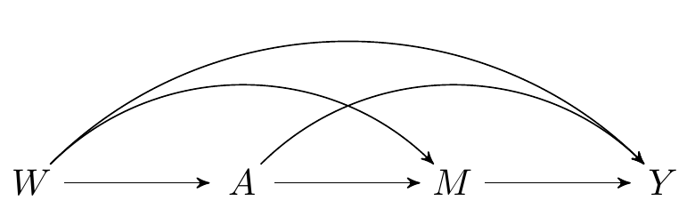
The data on a single observational unit can be represented \(O = (W, A, M, Y)\), with the data pooled across all participants denoted \(O_1, \ldots, O_n\), for a of \(n\) i.i.d. observations of \(O\). Recall the DAG from an earlier chapter, which represents the data-generating process:
Below, we demonstrate the construction of an ensemble learner based on a limited library of algorithms, including an intercept model, a main terms GLM, LASSO (\(\ell_1\)-penalized) regression, and random forest (ranger).
van der Laan, Mark J, Eric C Polley, and Alan E Hubbard. 2007. “Super Learner.”Statistical Applications in Genetics and Molecular Biology 6 (1).
Of course, there are many alternatives for learning algorithms to be included in such a modeling library. Feel free to explore!
6.2.2 Riesz representers
In a subset of the semi-parametric and double-machine learning literature, the weights in the EIF are sometimes referred to as Riesz representers. To understand why, let’s imagine that we want to estimate the total effect (i.e., the ATE) of a binary treatment \(A\) on some outcome \(Y\) accounting for confounders \(W\). Under standard identification assumptions, this effect is identified from the observed data as
Let’s denote \(Q(a,W) = \E[Y\mid A=a,W]\) and \(m(O;Q)\) as a continuous linear mapping of \(Q(a,W)\) and the observed data. In the case of the total effect, \(m(O;Q) = Q(1,W) - Q(0,W)\). We can then re-write the total effect as
\[
\E[m(O;Q)]\text{.}
\]
Now, consider that the total effect can equivalently be identified as
According to the Riesz representation theorem, if \(m(O;Q)\) is a continuous linear functional of \(Q\) (which it is), then there exists a unique function \(\alpha_0(W)\)–the so-called Riesz representer–such that
Thus, \(\frac{\I(A=1)}{\P(A=1 \mid W)} - \frac{\I(A=0)}{1 - \P(A=1 \mid W)}\) is the Riesz representer for estimating the total effect of \(A\) on \(Y\)!
While \(\alpha_0(W)\) for the total effect has a nice close-form solution that can be easily estimated with off-the-shelf software, this isn’t always the case. With that in mind, Chernozhukov et al. (2021) showed that the Riesz representer is the minimizer of the the so-called Riesz loss:
Chernozhukov, Victor, Whitney K Newey, Victor Quintas-Martinez, and Vasilis Syrgkanis. 2021. “Automatic Debiased Machine Learning via Riesz Regression.”arXiv Preprint arXiv:2104.14737.
This means that we can directly estimate \(\alpha_0(W)\) by minimizing the above loss function! For the case of mediation analysis, the methods we proposed in Liu et al. (2024) and implemented in crumble estimate Riesz representers of the type:
Liu, Richard, Nicholas T Williams, Kara E Rudolph, and Iván Dı́az. 2024. “General Targeted Machine Learning for Modern Causal Mediation Analysis.”arXiv Preprint arXiv:2408.14620.
crumble estimates this value (and others) for mediational effects directly by minimizing the Riesz loss with deep learning using torch. Much of this is abstracted away from the analyst, but we still need to specify some type of deep-learning architecture to use crumble. Here’s an example of a simple multilayer perceptron (MLP) with two hidden layers, each with 10 units, and a dropout rate of 0.1 which we create using the sequential_module() function from crumble.
Let’s use the crumble() function to estimate the natural direct and indirect effect.
We’ll use the ensemble of the intercept model, a main terms GLM, LASSO (\(\ell_1\)-penalized) regression, and random forest we defined above (ensemble) for the regression parameters
We’ll use the multilayer perceptron we defined above (mlp) to estimate the Riesz representers.
To indicate we want to estimate the natural (in)direct effects, we set effect = "N".
crumble was designed to also work with continuous exposures. Because of this, we need to specify the treatment regimes to create the contrasts for the (in)direct effects.
d0 and d1 are functions that return the treatment assignment under the two regimes. In our case, we want to estimate the effect of participating in a sports team, so we set d0 to always return 1 (i.e., no participation) and d1 to always return 0 (i.e., participation).
Want to learn more about specifying causal effects using these d functions? Check out the workshop, Beyond the ATE happening after this one!
6.4 Efficient estimation of the interventional (in)direct effects
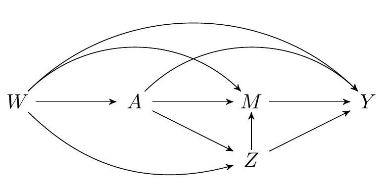
Since our knowledge of the system under study is incomplete, we might worry that one (or more) of the measured variables are not mediators, but, in fact, intermediate confounders affected by treatment. While the natural (in)direct effects are not identified in this setting, their interventional (in)direct counterparts are, as we saw in an earlier section. Recall that both types of effects are defined by static interventions on the treatment. The interventional effects are distinguished by their use of a stochastic intervention on the mediator to aid in their identification.
In our data example, we’ll consider the eating of snacks as a potential intermediate confounder, since one might reasonably hypothesize that participation on a sports team might subsequently affect snacking, which then could affect mediators like the amount of exercises and overweight status.
We can easily estimate the interventional direct and indirect effects by setting effect = "RI" and specifying the intermediate confounders in the moc argument.
# `R` packages for estimation of the causal (in)direct effects```{r}#| label: load-renv#| echo: false#| message: falserenv::autoload()library(here)```We'll now turn to working through a few examples of estimating the natural andinterventional direct and indirect effects. We will be using the [`crumble``R`package](https://cran.r-project.org/web/packages/crumble/index.html), whichprovides a unified framework for estimating many of the common mediationestimands, and supports high-dimensional exposures, mediators, andmediator-outcome confounders. However, many software implementations exist inthe `R` ecosystem for performing mediation analyses; notably, `crumble` washeavily inspired by [`medoutcon`](https://github.com/nhejazi/medoutcon),[`HDmediation`](https://github.com/nt-williams/HDmediation), and[`lcm`](https://github.com/nt-williams/lcm).As our running example, we'll use a simple data set from an observational studyof the relationship between BMI and kids' behavior, freely distributed with the[`mma` `R` package on CRAN](https://CRAN.R-project.org/package=mma). First,let's load the packages we'll be using and set a seed for reproducibility;then, load this data set and take a quick look.```{r}#| label: setup#| code-fold: falselibrary(crumble)library(mlr3extralearners)library(fastDummies)library(torch)set.seed(4235243)torch_manual_seed(657)# load and examine datadata(weight_behavior, package ="mma")# drop missing valuesweight_behavior <-na.omit(weight_behavior)# dummy code (aka one-hot-encode) factorsweight_behavior <-dummy_cols( weight_behavior, c("sex", "sports", "snack"),remove_selected_columns =TRUE,remove_first_dummy =TRUE)head(weight_behavior)```The documentation for the data set describes it as a "database obtained fromthe Louisiana State University Health Sciences Center, New Orleans, by Dr.Richard Scribner. He explored the relationship between BMI and kids' behaviorthrough a survey at children, teachers and parents in Grenada in 2014. Thisdata set includes 691 observations and 15 variables." Note that the data setcontained several observations with missing values, which we removed above tosimplify the demonstration of our analytic methods. In practice, we recommendinstead using appropriate corrections (e.g., imputation, inverse weighting) tofully take advantage of the observed data.Following the motivation of the original study, we focus on the causal effectsof participating in a sports team (`sports_2`) on the BMI of children (`bmi`),taking into consideration several mediators (`snack_2`, `exercises`); `c("age","sex_F", "tvhours")` are taken to be potential baseline confounders.## `crumble`: Flexible and general mediation analysis- `crumble` implements a one-step estimator of the natural, interventional, and organic (in)direct effect, as well as path-specific effects using recanting twins.- The estimator is capable of accommodating flexible modeling strategies (e.g., ensemble machine learning) for the initial estimation of nuisance parameters.- To this end, `crumble` integrates with the [`mlr3superlearner` R package](https://cran.r-project.org/package=mlr3superlearner).- The estimator uses cross-fitting of nuisance parameters. The data on a single observational unit can be represented $O = (W, A, M, Y)$,with the data pooled across all participants denoted $O_1, \ldots, O_n$, for aof $n$ i.i.d. observations of $O$. Recall the DAG [from an earlierchapter](#estimands), which represents the data-generating process:```{tikz}#| fig-cap: Directed acyclic graph under *no intermediate confounders* of the mediator-outcome relation affected by treatment\dimendef\prevdepth=0\pgfdeclarelayer{background}\pgfsetlayers{background,main}\usetikzlibrary{arrows,positioning}\tikzset{>=stealth',punkt/.style={rectangle,rounded corners,draw=black, very thick,text width=6.5em,minimum height=2em,text centered},pil/.style={->,thick,shorten <=2pt,shorten >=2pt,}}\newcommand{\Vertex}[2]{\node[minimum width=0.6cm,inner sep=0.05cm] (#2) at (#1) {$#2$};}\newcommand{\VertexR}[2]{\node[rectangle, draw, minimum width=0.6cm,inner sep=0.05cm] (#2) at (#1) {$#2$};}\newcommand{\ArrowR}[3]{ \begin{pgfonlayer}{background}\draw[->,#3] (#1) to[bend right=30] (#2);\end{pgfonlayer}}\newcommand{\ArrowL}[3]{ \begin{pgfonlayer}{background}\draw[->,#3] (#1) to[bend left=45] (#2);\end{pgfonlayer}}\newcommand{\EdgeL}[3]{ \begin{pgfonlayer}{background}\draw[dashed,#3] (#1) to[bend right=-45] (#2);\end{pgfonlayer}}\newcommand{\Arrow}[3]{ \begin{pgfonlayer}{background}\draw[->,#3] (#1) -- +(#2);\end{pgfonlayer}}\begin{tikzpicture} \Vertex{-4, 0}{W} \Vertex{0, 0}{M} \Vertex{-2, 0}{A} \Vertex{2, 0}{Y} \Arrow{W}{A}{black} \Arrow{A}{M}{black} \Arrow{M}{Y}{black} \ArrowL{W}{Y}{black} \ArrowL{A}{Y}{black} \ArrowL{W}{M}{black}\end{tikzpicture}```- In `crumble()`, $A$ is denoted `trt`, $Y$ is denoted `outcome`, $M$ is denoted `mediators`, and $W$ is denoted `covar`.## Estimating nuisance parameters- Recall that the one-step estimator can be thought of as a combination of a weighted estimator and a regression estimator. - We'd like to rely on flexible, data adaptive strategies for nuisance parameter estimation.- Doing so minimizes opportunities for model mis-specification to compromise our analytic conclusions.### Super learning- For the regression function parts of the EIF (e.g., $\E[Y\mid A,M,W]$),`crumble` uses the Super Learner algorithm for ensemble machine learning[@vdl2007super], which is implemented in the [`mlr3superlearner` R package](https://cran.r-project.org/package=mlr3superlearner).- Below, we demonstrate the construction of an ensemble learner based on a limited library of algorithms, including an intercept model, a main terms GLM, LASSO ($\ell_1$-penalized) regression, and random forest (`ranger`).```{r}#| code-fold: false#| eval: falseensemble <-list("mean","glm","cv_glmnet",list("ranger", num.trees =200))```- Of course, there are many alternatives for learning algorithms to be included in such a modeling library. Feel free to explore!### Riesz representersIn a subset of the semi-parametric and double-machine learning literature, theweights in the EIF are sometimes referred to as _Riesz representers_. Tounderstand why, let's imagine that we want to estimate the total effect (i.e.,the ATE) of a binary treatment $A$ on some outcome $Y$ accounting forconfounders $W$. Under standard identification assumptions, this effect isidentified from the observed data as$$\psi = \E[\E[Y\mid A= 1,W] - \E[Y\mid A= 0,W]]\text{.}$$Let's denote $Q(a,W) = \E[Y\mid A=a,W]$ and $m(O;Q)$ as a continuous linearmapping of $Q(a,W)$ and the observed data. In the case of the total effect,$m(O;Q) = Q(1,W) - Q(0,W)$. We can then re-write the total effect as$$\E[m(O;Q)]\text{.}$$Now, consider that the total effect can equivalently be identified as$$\E\bigg[\bigg\{\frac{\I(A=1)}{\P(A=1 \mid W)} - \frac{\I(A=0)}{1 - \P(A=1 \midW)}\bigg\}Y \bigg]\text{.}$$Let's denote $\frac{\I(A=1)}{\P(A=1 \mid W)} - \frac{\I(A=0)}{1 - \P(A=1 \midW)}$ as $\alpha_0(W)$. Then, $$\E[m(O;Q)] = \E[\alpha_0(W) \cdot Y]\text{.}$$According to the Riesz representation theorem, if $m(O;Q)$ is a continuouslinear functional of $Q$ (which it is), then there exists a unique function$\alpha_0(W)$--the so-called Riesz representer--such that$$\E[m(O;Q)] = \E[\alpha_0(W) \cdot Q(A,W)]\text{.}$$Using the tower rule, we have$$\begin{align*}\E[m(O;Q)] &= \E[\alpha_0(W) \cdot Y]\\&= \E\big[\E[\alpha_0(W) \cdot Y\mid A,W]\big]\\&= \E\big[\alpha_0(W) \cdot \E[Y\mid A,W]\big]\\& = \E[\alpha_0(W) \cdot Q(A,W)]\text{.}\end{align*}$$Thus, $\frac{\I(A=1)}{\P(A=1 \mid W)} - \frac{\I(A=0)}{1 - \P(A=1 \mid W)}$ isthe Riesz representer for estimating the total effect of $A$ on $Y$!While $\alpha_0(W)$ for the total effect has a nice close-form solution thatcan be easily estimated with off-the-shelf software, this isn't always thecase. With that in mind, @chernozhukov2021automatic showed that the Rieszrepresenter is the minimizer of the the so-called Riesz loss: $$\text{arg min}_\alpha \E[\alpha_0(W)^2 - 2\cdot m(O;\alpha)]\text{.}$$This means that we can directly estimate $\alpha_0(W)$ by minimizing the aboveloss function! For the case of mediation analysis, the methods we proposed in@liu2024general and implemented in `crumble` estimate Riesz representers of thetype:$$\frac{\I(A_i=1)}{\hat{\P}(A_i=1 \mid W_i)} \frac{\hat{\P}(M_i \mid A_i=0,W)_i}{\hat{\P}(M_i \mid A_i=1,W_i)} - \frac{\I(A=0)}{\hat{\P}(A_i=0 \mid W_i)}\text{.}$$`crumble` estimates this value (and others) for mediational effects directly byminimizing the Riesz loss with deep learning using `torch`. **Much of this isabstracted away from the analyst**, but we still need to specify some type ofdeep-learning architecture to use `crumble`. Here's an example of a simplemultilayer perceptron (MLP) with two hidden layers, each with 10 units, and adropout rate of 0.1 which we create using the `sequential_module()` functionfrom `crumble`.```{r}#| code-fold: false#| eval: falsemlp <-sequential_module(layers =2, hidden =10, dropout =0.1)```## Efficient estimation of the natural (in)direct effectsTo start, we will consider estimation of the *natural* direct and indirecteffects, which, we recall, are defined as follows$$ \E[Y_{1,M_1} - Y_{0,M_0}] = \underbrace{\E[Y_{\color{red}{1},\color{blue}{M_1}} - Y_{\color{red}{1},\color{blue}{M_0}}]}_{\text{natural indirect effect}} + \underbrace{\E[Y_{\color{blue}{1},\color{red}{M_0}} - Y_{\color{blue}{0},\color{red}{M_0}}]}_{\text{natural direct effect}}.$$Let's use the `crumble()` function to estimate the natural direct and indirect effect. - We'll use the ensemble of the intercept model, a main terms GLM, LASSO ($\ell_1$-penalized) regression, and random forest we defined above (`ensemble`) for the regression parameters- We'll use the multilayer perceptron we defined above (`mlp`) to estimate the Riesz representers.- To indicate we want to estimate the natural (in)direct effects, we set`effect = "N"`. - `crumble` was designed to also work with continuous exposures. Because of this, we need to specify the treatment regimes to create the contrasts for the (in)direct effects. - `d0` and `d1` are functions that return the treatment assignment under the two regimes. In our case, we want to estimate the effect of participating in a sports team, so we set `d0` to always return 1 (i.e., no participation) and `d1` to always return 0 (i.e., participation). - Want to learn more about specifying causal effects using these `d` functions? Check out the workshop, _Beyond the ATE_ happening after this one!```{r}#| label: natural-os#| code-fold: false#| eval: false# compute one-step estimates of the natural effectscrumble(data = weight_behavior,trt ="sports_2",outcome ="bmi",covar =c("age", "sex_F", "tvhours"),mediators =c("snack_2", "exercises"),d0 =function(data, trt) rep(1, nrow(data)),d1 =function(data, trt) rep(0, nrow(data)),effect ="N",learners = ensemble,nn_module = mlp,control =crumble_control(crossfit_folds =1L, epochs =10L, learning_rate =0.01))# ✔ Fitting outcome regressions... 1/1 folds [5.4s]# ✔ Computing alpha n density ratios... 1/1 folds [7s]## ══ Results `crumble()` ════════════════════════════════════════════════════════════════## ── Direct Effect# Estimate: -1.08# Std. error: 0.26# 95% Conf. int.: -1.6, -0.57## ── Indirect Effect# Estimate: 0.06# Std. error: 0.05# 95% Conf. int.: -0.05, 0.16## ── Average Treatment Effect# Estimate: -1.03# Std. error: 0.3# 95% Conf. int.: -1.61, -0.44```## Efficient estimation of the interventional (in)direct effectsSince our knowledge of the system under study is incomplete, we might worrythat one (or more) of the measured variables are not mediators, but, in fact,intermediate confounders affected by treatment. While the natural (in)directeffects are not identified in this setting, their interventional (in)directcounterparts are, as we saw in an earlier section. Recall that both types ofeffects are defined by static interventions on the treatment. Theinterventional effects are distinguished by their use of a stochasticintervention on the mediator to aid in their identification.```{tikz}#| fig-cap: Directed acyclic graph under intermediate confounders of the mediator-outcome relation affected by treatment\dimendef\prevdepth=0\pgfdeclarelayer{background}\pgfsetlayers{background,main}\usetikzlibrary{arrows,positioning}\tikzset{>=stealth',punkt/.style={rectangle,rounded corners,draw=black, very thick,text width=6.5em,minimum height=2em,text centered},pil/.style={->,thick,shorten <=2pt,shorten >=2pt,}}\newcommand{\Vertex}[2]{\node[minimum width=0.6cm,inner sep=0.05cm] (#2) at (#1) {$#2$};}\newcommand{\VertexR}[2]{\node[rectangle, draw, minimum width=0.6cm,inner sep=0.05cm] (#2) at (#1) {$#2$};}\newcommand{\ArrowR}[3]{ \begin{pgfonlayer}{background}\draw[->,#3] (#1) to[bend right=30] (#2);\end{pgfonlayer}}\newcommand{\ArrowL}[3]{ \begin{pgfonlayer}{background}\draw[->,#3] (#1) to[bend left=45] (#2);\end{pgfonlayer}}\newcommand{\EdgeL}[3]{ \begin{pgfonlayer}{background}\draw[dashed,#3] (#1) to[bend right=-45] (#2);\end{pgfonlayer}}\newcommand{\Arrow}[3]{ \begin{pgfonlayer}{background}\draw[->,#3] (#1) -- +(#2);\end{pgfonlayer}}\begin{tikzpicture} \Vertex{0, -1}{Z} \Vertex{-4, 0}{W} \Vertex{0, 0}{M} \Vertex{-2, 0}{A} \Vertex{2, 0}{Y} \ArrowR{W}{Z}{black} \Arrow{Z}{M}{black} \Arrow{W}{A}{black} \Arrow{A}{M}{black} \Arrow{M}{Y}{black} \Arrow{A}{Z}{black} \Arrow{Z}{Y}{black} \ArrowL{W}{Y}{black} \ArrowL{A}{Y}{black} \ArrowL{W}{M}{black}\end{tikzpicture}```Recall that the interventional (in)direct effects are defined via the decomposition:$$ \E[Y_{1,G_1} - Y_{0,G_0}] = \underbrace{\E[Y_{\color{red}{1},\color{blue}{G_1}} - Y_{\color{red}{1},\color{blue}{G_0}}]}_{\text{interventional indirect effect}} + \underbrace{\E[Y_{\color{blue}{1},\color{red}{G_0}} - Y_{\color{blue}{0},\color{red}{G_0}}]}_{\text{interventional direct effect}}$$- In our data example, we'll consider the eating of snacks as a potential intermediate confounder, since one might reasonably hypothesize that participation on a sports team might subsequently affect snacking, which then could affect mediators like the amount of exercises and overweight status.\- We can easily estimate the interventional direct and indirect effects by setting `effect = "RI"` and specifying the intermediate confounders in the`moc` argument.```{r}#| code-fold: false#| eval: false# compute one-step estimates of the interventional effectscrumble(data = weight_behavior,trt ="sports_2",outcome ="bmi",covar =c("age", "sex_F", "tvhours"),mediators ="exercises",moc ="snack_2",d0 =function(data, trt) rep(1, nrow(data)),d1 =function(data, trt) rep(0, nrow(data)),effect ="RI",learners = ensemble,nn_module = mlp,control =crumble_control(crossfit_folds =1L, epochs =10L, learning_rate =0.01))# ✔ Permuting Z-prime variables... 1/1 tasks [1.3s]# ✔ Fitting outcome regressions... 1/1 folds [7.1s]# ✔ Computing alpha r density ratios... 1/1 folds [13.3s]## ══ Results `crumble()` ════════════════════════════════════════════════════════════════## ── Randomized Direct Effect# Estimate: -1.12# Std. error: 0.43# 95% Conf. int.: -1.97, -0.27## ── Randomized Indirect Effect# Estimate: 0# Std. error: 0.03# 95% Conf. int.: -0.05, 0.05```