Chapter 6 Construction of a semiparametric efficient estimator for the NDE (a.k.a. the one-step estimator)
- Here we show the detail of how to construct an estimator for the NDE for illustration, but the construction of this estimator is a bit involved and may be complex in daily research practice
- For practice, we will teach you how to use our packages medoutcon (and medshift, as detailed in the extra material) for automatic implementation of these estimators of the NDE and other parameters
First, we need to introduce some notation to describe the EIF for the NDE
- Let \(Q(M, W)\) denote \(\E(Y\mid A=1, M, W) - \E(Y\mid A=0, M, W)\)
- We can now introduce the semiparametric efficient estimator:
\[\begin{align*} \hat{\psi} &= \frac{1}{n} \sum_{i=1}^n \color{RoyalBlue}{\bigg\{ \frac{\I(A_i=1)}{\hat{\P}(A_i=1 \mid W_i)} \frac{\hat{\P}(M_i \mid A_i=0,W)_i}{\hat{\P}(M_i \mid A_i=1,W_i)} - \frac{\I(A=0)}{\hat{\P}(A_i=0 \mid W_i)}\bigg\}} \color{Goldenrod}{[Y_i - \hat{\E}(Y\mid A_i,M_i,W_i)]} \\ &+ \frac{1}{n} \sum_{i=1}^n \color{RoyalBlue}{\frac{\I(A=0)}{\P(A=0 \mid W)}} \color{Goldenrod}{\big\{ \hat{Q}(M_i,W_i) - \hat{\E}[\hat{Q}(M_i,W_i) \mid W_i, A_i = 0] \big\}} \\ &+ \frac{1}{n} \sum_{i=1}^n \color{Goldenrod}{ \hat{\E}[\hat{Q}(M_i,W_i) \mid W_i,A_i=0]} \end{align*}\]
- In this estimator, you can recognize elements from the G-computation estimator
and the weighted estimators:
- The third line is the G-computation estimator
- The second line is a centered version of the second weighted estimator
- The first line is a centered version of the first weighted estimator
- Estimating \(\P(M\mid A, W)\) is a very challenging problem when \(M\) is high-dimensional. But, since we have the ratio of these conditional densities, we can re-paramterize using Bayes’ rule to get something that is easier to compute: \[\begin{equation*} \frac{\P(M \mid A=0, W)}{\P(M \mid A=1,W)} = \frac{\P(A = 0 \mid M, W) \P(A=1 \mid W)}{\P(A = 1 \mid M, W) \P(A=0 \mid W)} \ . \end{equation*}\]
Thus we can change the expression of the estimator a bit as follows. First, some more notation that will be useful later:
- Let \(g(a\mid w)\) denote \(\P(A=a\mid W=w)\)
- Let \(e(a\mid m, w)\) denote \(\P(A=a\mid M=m, W=w)\)
- Let \(b(a, m, w)\) denote \(\E(Y\mid A=a, M=m, W=w)\)
- The quantity being averaged can be re-expressed as follows
\[\begin{align*} & \color{RoyalBlue}{\bigg\{ \frac{\I(A=1)}{g(0\mid W)} \frac{e(0\mid M,W)}{e(1\mid M,W)} - \frac{\I(A=0)}{g(0\mid W)}\bigg\}} \times \color{Goldenrod}{[Y - b(A,M,W)]} \\ &+ \color{RoyalBlue}{\frac{\I(A=0)}{g(0\mid W)}} \color{Goldenrod}{\big\{Q(M,W) - \E[Q(M,W) \mid W, A=0] \big\}} \\ &+ \color{Goldenrod}{\E[Q(M,W) \mid W, A=0]} \end{align*}\]
6.1 How to compute the one-step estimator (akin to Augmented IPW)
First we will generate some data:
mean_y <- function(m, a, w) abs(w) + a * m
mean_m <- function(a, w)plogis(w^2 - a)
pscore <- function(w) plogis(1 - abs(w))

w_big <- runif(1e6, -1, 1)
trueval <- mean((mean_y(1, 1, w_big) - mean_y(1, 0, w_big)) * mean_m(0, w_big)
                + (mean_y(0, 1, w_big) - mean_y(0, 0, w_big)) *
                  (1 - mean_m(0, w_big)))

n <- 1000
w <- runif(n, -1, 1)
a <- rbinom(n, 1, pscore(w))
m <- rbinom(n, 1, mean_m(a, w))
y <- rnorm(n, mean_y(m, a, w))
Recall that the semiparametric efficient estimator can be computed in the following steps:
- Fit models for \(g(a\mid w)\), \(e(a\mid m, w)\), and \(b(a, m, w)\)
- In this example we will use Generalized Additive Models for tractability
- In applied settings we recommend using an ensemble of data-adaptive regression algorithms, such as the Super Learner (van der Laan, Polley and Hubbard, 2007)
library(mgcv)
## fit model for E(Y | A, W)
b_fit <- gam(y ~ m:a + s(w, by = a))
## fit model for P(A = 1 | M, W)
e_fit <- gam(a ~ m + w + s(w, by = m), family = binomial)
## fit model for P(A = 1 | W)
g_fit <- gam(a ~ w, family = binomial)- Compute predictions \(g(1\mid w)\), \(g(0\mid w)\), \(e(1\mid m, w)\), \(e(0\mid m, w)\),\(b(1, m, w)\), \(b(0, m, w)\), and \(b(a, m, w)\)
## Compute P(A = 1 | W)
g1_pred <- predict(g_fit, type = 'response')
## Compute P(A = 0 | W)
g0_pred <- 1 - g1_pred
## Compute P(A = 1 | M, W)
e1_pred <- predict(e_fit, type = 'response')
## Compute P(A = 0 | M, W)
e0_pred <- 1 - e1_pred
## Compute E(Y | A = 1, M, W)
b1_pred <- predict(b_fit, newdata = data.frame(a = 1, m, w))
## Compute E(Y | A = 0, M, W)
b0_pred <- predict(b_fit, newdata = data.frame(a = 0, m, w))
## Compute E(Y | A, M, W)
b_pred <- predict(b_fit)- Compute \(Q(M, W)\), fit a model for \(\E[Q(M,W) \mid W,A]\), and predict at \(A=0\)
## Compute Q(M, W)
pseudo <- b1_pred - b0_pred
## Fit model for E[Q(M, W) | A, W]
q_fit <- gam(pseudo ~ a + w + s(w, by = a))
## Compute E[Q(M, W) | A = 0, W]
q_pred <- predict(q_fit, newdata = data.frame(a = 0, w = w))- Estimate the weights \[\begin{equation*} \color{RoyalBlue}{\bigg\{ \frac{\I(A=1)}{g(0\mid W)} \frac{e(0 \mid M,W)}{e(1 \mid M,W)} - \frac{\I(A=0)}{g(0\mid W)} \bigg\}} \end{equation*}\] using the above predictions:
ip_weights <- a / g0_pred * e0_pred / e1_pred - (1 - a) / g0_pred- Compute the uncentered EIF:
eif <- ip_weights * (y - b_pred) + (1 - a) / g0_pred * (pseudo - q_pred) +
q_pred- The one step estimator is the mean of the uncentered EIF
## One-step estimator
mean(eif)
#> [1] 0.50127
6.2 Performance of the one-step estimator in a small simulation study
First, we create a wrapper around the estimator
one_step <- function(y, m, a, w) {
  b_fit <- gam(y ~ m:a + s(w, by = a))
  e_fit <- gam(a ~ m + w + s(w, by = m), family = binomial)
  g_fit <- gam(a ~ w, family = binomial)
  g1_pred <- predict(g_fit, type = 'response')
  g0_pred <- 1 - g1_pred
  e1_pred <- predict(e_fit, type = 'response')
  e0_pred <- 1 - e1_pred
  b1_pred <- predict(
    b_fit, newdata = data.frame(a = 1, m, w), type = 'response'
  )
  b0_pred <- predict(
    b_fit, newdata = data.frame(a = 0, m, w), type = 'response'
  )
  b_pred  <- predict(b_fit, type = 'response')
  pseudo <- b1_pred - b0_pred
  q_fit <- gam(pseudo ~ a + w + s(w, by = a))
  q_pred <- predict(q_fit, newdata = data.frame(a = 0, w = w))
  ip_weights <- a / g0_pred * e0_pred / e1_pred - (1 - a) / g0_pred
  eif <- ip_weights * (y - b_pred) + (1 - a) / g0_pred *
    (pseudo - q_pred) + q_pred
  return(mean(eif))
}
Let us first examine the bias
- The true value is:
w_big <- runif(1e6, -1, 1)
trueval <- mean((mean_y(1, 1, w_big) - mean_y(1, 0, w_big)) * mean_m(0, w_big)
  + (mean_y(0, 1, w_big) - mean_y(0, 0, w_big)) * (1 - mean_m(0, w_big)))
print(trueval)
#> [1] 0.5804- Bias simulation
estimate <- lapply(seq_len(1000), function(iter) {
  n <- 1000
  w <- runif(n, -1, 1)
  a <- rbinom(n, 1, pscore(w))
  m <- rbinom(n, 1, mean_m(a, w))
  y <- rnorm(n, mean_y(m, a, w))
  estimate <- one_step(y, m, a, w)
  return(estimate)
})
estimate <- do.call(c, estimate)

hist(estimate)
abline(v = trueval, col = "red", lwd = 4)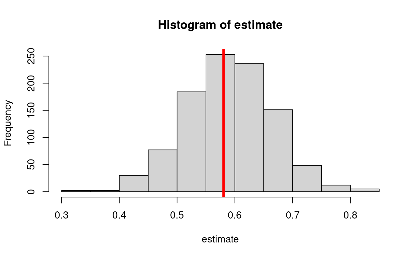
- And now the confidence intervals:
cis <- cbind(
  estimate - qnorm(0.975) * sd(estimate),
  estimate + qnorm(0.975) * sd(estimate)
)

ord <- order(rowSums(cis))
lower <- cis[ord, 1]
upper <- cis[ord, 2]
curve(trueval + 0 * x,
  ylim = c(0, 1), xlim = c(0, 1001), lwd = 2, lty = 3, xaxt = "n",
  xlab = "", ylab = "Confidence interval", cex.axis = 1.2, cex.lab = 1.2
)
for (i in 1:1000) {
  clr <- rgb(0.5, 0, 0.75, 0.5)
  if (upper[i] < trueval || lower[i] > trueval) clr <- rgb(1, 0, 0, 1)
  points(rep(i, 2), c(lower[i], upper[i]), type = "l", lty = 1, col = clr)
}
text(450, 0.10, "n=1000 repetitions = 1000 ", cex = 1.2)
text(450, 0.01, paste0(
  "Coverage probability = ",
  mean(lower < trueval & trueval < upper), "%"
), cex = 1.2)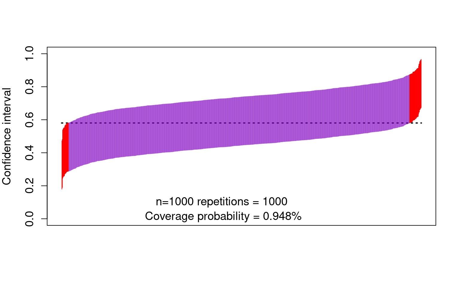
6.3 A note about targeted minimum loss-based estimation (TMLE)
- The above estimator is great because it allows us to use data-adaptive regression to avoid bias, while allowing the computation of correct standard errors
- This estimator has a problem, though:
- It can yield answers outside of the bounds of the parameter space
- E.g., if \(Y\) is binary, it could yield direct and indirect effects outside of \([-1,1]\)
- To solve this, you can compute a TMLE instead (implemented in the R packages, coming up)
6.4 A note about cross-fitting
- When using data-adaptive regression estimators, it is recommended to use cross-fitted estimators
- Cross-fitting is similar to cross-validation:
- Randomly split the sample into K (e.g., K=10) subsets of equal size
- For each of the 9/10ths of the sample, fit the regression models
- Use the out-of-sample fit to predict in the remaining 1/10th of the sample
- Cross-fitting further reduces the bias of the estimators
- Cross-fitting aids in guaranteeing the correctness of the standard errors and confidence intervals
- Cross-fitting is implemented by default in the R packages that you will see next