Chapter 6 Using the EIF to construct an estimator: the case of the natural direct effect
6.1 Natural direct effect
Recall:
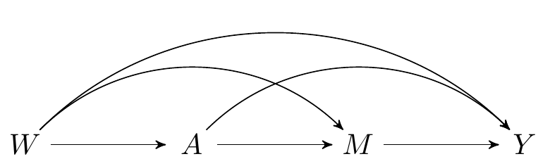
FIGURE 2.1: Directed acyclic graph under no intermediate confounders of the mediator-outcome relation affected by treatment
Assuming a binary \(A\), we define the natural direct effect as: \[NDE = E(Y_{1,M_{0}} - Y_{0,M_{0}}),\]
and the natural indirect effect as: \[NIE = E(Y_{1,M_{1}} - Y_{1,M_{0}}).\]
The observed data is \(O=(W, A, M, Y)\)
This SCM is represented in the above DAG and the following causal models: \[\begin{align*} W & = f_W(U_W)\\ A & = f_A(W, U_A)\\ M & = f_M(W, A, U_M)\\ Y & = f_Y(W, A, M, U_Y), \end{align*}\] where \((U_W, U_A,U_M, U_Y)\) are exogenous random errors.
We assume - \(A\) is a single binary randomized treatment (and thus \(A = f_A(U_A)\)) - \(M\) is a single binary mediator - There are no restrictions on the distribution of \(W\) or \(Y\)
Recall that we need to assume the following to identify the above caual effects from our observed data:
- \(A \indep Y_{a,m} \mid W\)
- \(M \indep Y_{a,m} \mid W, A\)
- \(A \indep M_a \mid W\)
- \(M_0 \indep Y_{1,m} \mid W\)
- and positivity assumptions
Then, the NDE is identified as \[\begin{equation*} \psi(\P) = \E[\E\{\E(Y \mid A=1, M, W) - \E(Y \mid A=0, M, W)\mid A=0,W\}] \end{equation*}\]
6.1.1 The efficient influence function for the NDE
- For illustration, we will first present how to construct an estimator of the NDE that uses the EIF ``by hand’’
- For other parameters, we will teach you how to use our packages medoutcon and medshift
First, we need to introduce some notation to describe the EIF for the NDE
Let \(Q(M, W)\) denote \(\E(Y\mid A=1, M, W) - \E(Y\mid A=0, M, W)\)
We can now introduce the EIF: \[\begin{align*} D(O) &= \color{RoyalBlue}{\bigg\{ \frac{I(A=1)}{\P(A=1\mid W)}\frac{\P(M\mid A=0,W)}{\P(M\mid A=1,W)} - \frac{I(A=0)}{\P(A=0\mid W)}\bigg\}} \times \color{Goldenrod}{[Y-\E(Y\mid A,M,W)]} \\ &+ \color{RoyalBlue}{\frac{I(A=0)}{\P(A=0\mid W)}}\color{Goldenrod}{\big\{Q(M,W) - \E[Q(M,W) | W,A=0] \big\}}\\ &+ \color{Goldenrod}{\E[Q(M,W) | W,A=0] - \psi(\P)} \end{align*}\]
In this EIF, you can recognize elements from the g-computation estimator and the weighted estimator:
- \(Q(M, W)\) shows up in the g-computation estimator
- The weights in blue in the first part of the EIF are used in the weighted estimator
Estimating \(\P(M\mid A, W)\) is a really hard problem when \(M\) is high-dimensional. But, since we have the ratio of these conditional densitities, we can reparamterize using Bayes rule to get something that is easier to compute:
\[\begin{equation*} \frac{\P(M\mid A=0,W)}{\P(M\mid A=1,W)} = \frac{\P(A = 0 \mid M, W) \P(A=1 \mid W)}{\P(A = 1 \mid M, W)\P(A=0 \mid W)}. \end{equation*}\]
Thus we can change the expression of the EIF a bit as follows. First, some more notation that will be useful later:
- Let \(g(a\mid w)\) denote \(\P(A=a\mid W=w)\)
- Let \(e(a\mid m, w)\) denote \(\P(A=a\mid M=m, W=w)\)
- Let \(b(a, m, w)\) denote \(\E(Y\mid A=a, M=m, W=w)\)
- The EIF is
\[\begin{align*} D(O) &= \color{RoyalBlue}{\bigg\{ \frac{I(A=1)}{g(0\mid W)}\frac{e(0\mid M,W)}{e(1\mid M,W)} - \frac{I(A=0)}{g(0\mid W)}\bigg\}} \times \color{Goldenrod}{[Y-b(A,M,W)]} \\ &+ \color{RoyalBlue}{\frac{I(A=0)}{g(0\mid W)}}\color{Goldenrod}{\big\{Q(M,W) - \E[Q(M,W) | W,A=0] \big\}}\\ &+ \color{Goldenrod}{\E[Q(M,W) | W,A=0] - \psi(\P)} \end{align*}\]
6.1.2 How to compute the one-step estimator (akin to Augmented IPW)
First we will generate some data:
mean_y <- function(m, a, w) abs(w) + a * m
mean_m <- function(a, w)plogis(w^2 - a)
pscore <- function(w) plogis(1 - abs(w))

w_big <- runif(1e6, -1, 1)
trueval <- mean((mean_y(1, 1, w_big) - mean_y(1, 0, w_big)) * mean_m(0, w_big)
                + (mean_y(0, 1, w_big) - mean_y(0, 0, w_big)) *
                  (1 - mean_m(0, w_big)))

n <- 1000
w <- runif(n, -1, 1)
a <- rbinom(n, 1, pscore(w))
m <- rbinom(n, 1, mean_m(a, w))
y <- rnorm(n, mean_y(m, a, w))
Recall that the one-step estimator is defined as the bias-corrected g-computation estimator: \[\begin{equation*} \psi(\hat \P) + \frac{1}{n}\sum_{i=1}^n D(O;\hat \P_i) \end{equation*}\]
Can be computed in the following steps:
- Fit models for \(g(a\mid w)\), \(e(a\mid m, w)\), and \(b(a, m, w)\)
- In this example we will use Generalized Additive Models for tractability
- In applied settings we recommend using an ensemble of data-adaptive regression algorithms, such as the Super Learner (van der Laan, Polley, and Hubbard 2007)
library(mgcv)
## fit model for E(Y | A, W)
b_fit <- gam(y ~ m:a + s(w, by = a))
## fit model for P(A = 1 | M, W)
e_fit <- gam(a ~ m + w + s(w, by = m), family = binomial)
## fit model for P(A = 1 | W)
g_fit <- gam(a ~ w, family = binomial)- Compute predictions \(g(1\mid w)\), \(g(0\mid w)\), \(e(1\mid m, w)\), \(e(0\mid m, w)\),\(b(1, m, w)\), \(b(0, m, w)\), and \(b(a, m, w)\)
## Compute P(A = 1 | W)
g1_pred <- predict(g_fit, type = 'response')
## Compute P(A = 0 | W)
g0_pred <- 1 - g1_pred
## Compute P(A = 1 | M, W)
e1_pred <- predict(e_fit, type = 'response')
## Compute P(A = 0 | M, W)
e0_pred <- 1 - e1_pred
## Compute E(Y | A = 1, M, W)
b1_pred <- predict(b_fit, newdata = data.frame(a = 1, m, w))
## Compute E(Y | A = 0, M, W)
b0_pred <- predict(b_fit, newdata = data.frame(a = 0, m, w))
## Compute E(Y | A, M, W)
b_pred <- predict(b_fit)- Compute \(Q(M, W)\), fit a model for \(\E[Q(M,W) | W,A]\), and predict at \(A=0\)
## Compute Q(M, W)
pseudo <- b1_pred - b0_pred
## Fit model for E[Q(M, W) | A, W]
q_fit <- gam(pseudo ~ a + w + s(w, by = a))
## Compute E[Q(M, W) | A = 0, W]
q_pred <- predict(q_fit, newdata = data.frame(a = 0, w = w))- Estimate the weights \[\begin{equation*} \color{RoyalBlue}{\bigg\{ \frac{I(A=1)}{g(0\mid W)}\frac{e(0\mid M,W)}{e(1\mid M,W)} - \frac{I(A=0)}{g(0\mid W)}\bigg\}} \end{equation*}\] using the above predictions:
- Compute the uncentered EIF:
- The one step estimator is the mean of the uncentered EIF
6.1.3 Performance of the one-step estimator in a small simulation study
First, we create a wrapper around the estimator
one_step <- function(y, m, a, w) {
b_fit <- gam(y ~ m:a + s(w, by = a))
e_fit <- gam(a ~ m + w + s(w, by = m), family = binomial)
g_fit <- gam(a ~ w, family = binomial)
g1_pred <- predict(g_fit, type = 'response')
g0_pred <- 1 - g1_pred
e1_pred <- predict(e_fit, type = 'response')
e0_pred <- 1 - e1_pred
b1_pred <- predict(b_fit, newdata = data.frame(a = 1, m, w),
type = 'response')
b0_pred <- predict(b_fit, newdata = data.frame(a = 0, m, w),
type = 'response')
b_pred <- predict(b_fit, type = 'response')
pseudo <- b1_pred - b0_pred
q_fit <- gam(pseudo ~ a + w + s(w, by = a))
q_pred <- predict(q_fit, newdata = data.frame(a = 0, w = w))
ip_weights <- a / g0_pred * e0_pred / e1_pred - (1 - a) / g0_pred
eif <- ip_weights * (y - b_pred) + (1 - a) / g0_pred * (pseudo - q_pred) +
  q_pred
return(mean(eif))
}Let us first examine the bias
- The true value is:
w_big <- runif(1e6, -1, 1)
trueval <- mean((mean_y(1, 1, w_big) - mean_y(1, 0, w_big)) * mean_m(0, w_big) +
  (mean_y(0, 1, w_big) - mean_y(0, 0, w_big)) * (1 - mean_m(0, w_big)))
print(trueval)
#> [1] 0.58061- Bias simulation
estimate <- lapply(seq_len(1000), function(iter) {
  n <- 1000
  w <- runif(n, -1, 1)
  a <- rbinom(n, 1, pscore(w))
  m <- rbinom(n, 1, mean_m(a, w))
  y <- rnorm(n, mean_y(m, a, w))
  estimate <- one_step(y, m, a, w)
  return(estimate)
})
estimate <- do.call(c, estimate)

hist(estimate)
abline(v = trueval, col = "red", lwd = 4)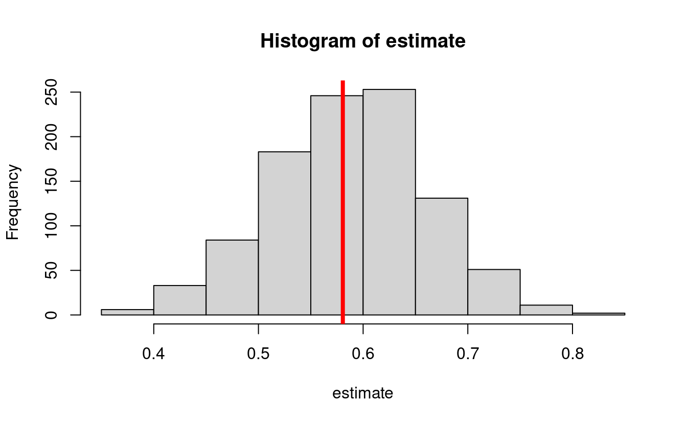
- And now the confidence intervals:
cis <- cbind(
  estimate - qnorm(0.975) * sd(estimate),
  estimate + qnorm(0.975) * sd(estimate)
)

ord <- order(rowSums(cis))
lower <- cis[ord, 1]
upper <- cis[ord, 2]
curve(trueval + 0 * x,
  ylim = c(0, 1), xlim = c(0, 1001), lwd = 2, lty = 3, xaxt = "n",
  xlab = "", ylab = "Confidence interval", cex.axis = 1.2, cex.lab = 1.2
)
for (i in 1:1000) {
  clr <- rgb(0.5, 0, 0.75, 0.5)
  if (upper[i] < trueval || lower[i] > trueval) clr <- rgb(1, 0, 0, 1)
  points(rep(i, 2), c(lower[i], upper[i]), type = "l", lty = 1, col = clr)
}
text(450, 0.10, "n=1000 repetitions = 1000 ", cex = 1.2)
text(450, 0.01, paste0(
  "Coverage probability = ",
  mean(lower < trueval & trueval < upper), "%"
), cex = 1.2)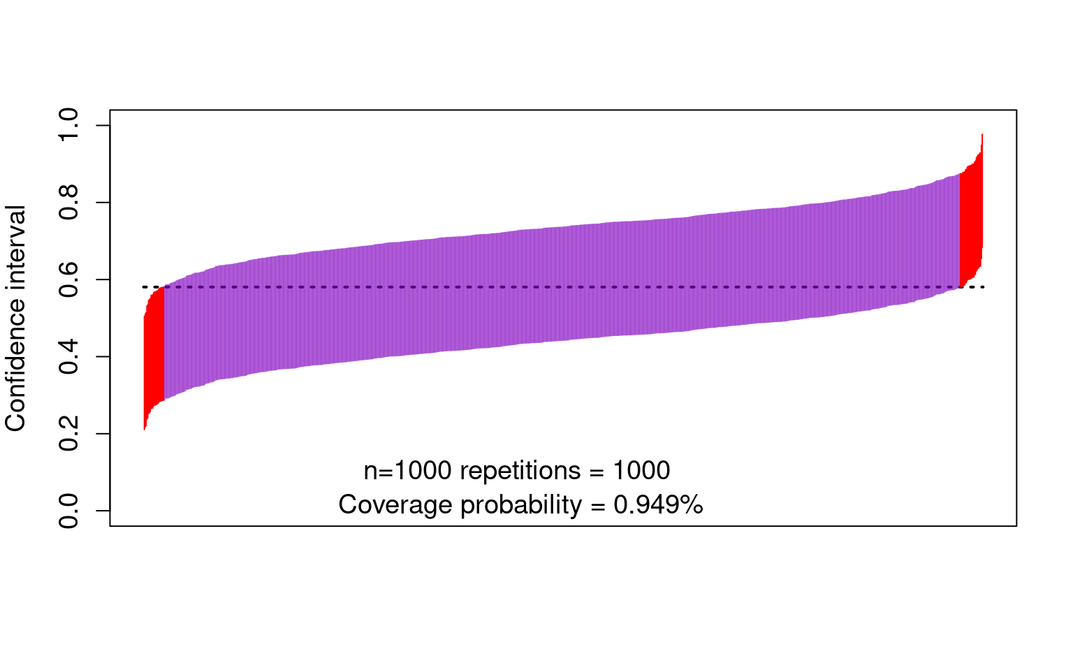
6.1.4 A note about targeted minimum loss-based estimation (TMLE)
- The above estimator is great because it allows us to use data-adaptive regression to avoid bias, while allowing the computation of correct standard errors
- This estimator has one problem:
- It can yield answers outside of the bounds of the parameter space
- E.g., if \(Y\) is binary, it could yield direct and indirect effects outside of \([-1,1]\)
- To solve this, you can compute a TMLE instead (implemented in the R packages, coming up)
6.1.5 A note about cross-fitting
- When using data-adaptive regression estimators, it is recommended to use cross-fitted estimators
- Cross-fitting is similar to cross-validation:
- Randomly split the sample into K (e.g., K=10) subsets of equal size
- For each of the 9/10ths of the sample, fit the regression models
- Use the out-of-sample fit to predict in the remaining 1/10th of the sample
- Cross-fitting further reduces the bias of the estimators
- Cross-fitting aids in guaranteeing the correctness of the standard errors and confidence intervals
- Cross-fitting is implemented by default in the R packages that you will see next