Chapter 7 `R` packages for estimation of the causal (in)direct effects

We’ll now turn to working through a few examples of estimating the natural, interventional, and stochastic direct and indirect effects. As our running example, we’ll a simple data set from an observational study of the relationship between BMI and kids’ behavior, freely distributed with the mma R package on CRAN. First, let’s load the packages we’ll be using and set a seed; then, load this data set and take a quick look

library(tidyverse)
library(sl3)
library(medoutcon)
library(medshift)
library(mma)
set.seed(429153)

# load and examine data
data(weight_behavior)
dim(weight_behavior)
#> [1] 691  15

# drop missing values
weight_behavior <- weight_behavior %>%
  drop_na() %>%
  as_tibble()
weight_behavior
#> # A tibble: 567 × 15
#>     bmi   age sex   race  numpeople   car gotosch snack tvhours cmpthours
#>   <dbl> <dbl> <fct> <fct>     <int> <int> <fct>   <fct>   <dbl>     <dbl>
#> 1  18.2  12.2 F     OTHER         5     3 2       1           4         0
#> 2  22.8  12.8 M     OTHER         4     3 2       1           4         2
#> 3  25.6  12.1 M     OTHER         2     3 2       1           0         2
#> 4  15.1  12.3 M     OTHER         4     1 2       1           2         1
#> 5  23.0  11.8 M     OTHER         4     1 1       1           4         3
#> # … with 562 more rows, and 5 more variables: cellhours <dbl>, sports <fct>,
#> #   exercises <int>, sweat <int>, overweigh <dbl>

The documentation for the data set describes it as a “database obtained from the Louisiana State University Health Sciences Center, New Orleans, by Dr. Richard Scribner. He explored the relationship between BMI and kids’ behavior through a survey at children, teachers and parents in Grenada in 2014. This data set includes 691 observations and 15 variables.” Note that the data set contained several observations with missing values, which we removed above to simplify the demonstration of our analytic methods. In practice, we recommend instead using appropriate corrections (e.g., imputation, inverse weighting) to fully take advantage of the observed data.

Following the motivation of the original study, we focus on the causal effects of participating in a sports team (sports) on the BMI of children (bmi), taking into consideration several mediators (snack, exercises, overweigh); all other measured covariates are taken to be potential baseline confounders.

7.1 `medoutcon`: Natural and interventional (in)direct effects

The data on a single observational unit can be represented \(O = (W, A, M, Y)\), with the data pooled across all participants denoted \(O_1, \ldots, O_n\), for a of \(n\) i.i.d. observations of \(O\). Recall the DAG from an earlier chapter, which represents the data-generating process:

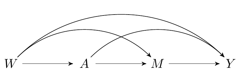
FIGURE 2.1: Directed acyclic graph under no intermediate confounders of the mediator-outcome relation affected by treatment

7.1.1 Natural (in)direct effects

To start, we will consider estimation of the natural direct and indirect effects, which, we recall, are defined as follows \[\begin{equation*} \E[Y_{1,M_1} - Y_{0,M_0}] = \underbrace{\E[Y_{\color{red}{1},\color{blue}{M_1}} - Y_{\color{red}{1},\color{blue}{M_0}}]}_{\text{natural indirect effect}} + \underbrace{\E[Y_{\color{blue}{1},\color{red}{M_0}} - Y_{\color{blue}{0},\color{red}{M_0}}]}_{\text{natural direct effect}}. \end{equation*}\]

Our medoutcon R package (Hejazi, Dı́az, and Rudolph 2022; Hejazi, Rudolph, and Dı́az 2022), which accompanies Dı́az et al. (2020), implements one-step and TML estimators of both the natural and interventional (in)direct effects.
Both types of estimators are capable of accommodating flexible modeling strategies (e.g., ensemble machine learning) for the initial estimation of nuisance parameters.
The medoutcon R package uses cross-validation in initial estimation: this results in cross-validated (or “cross-fitted”) one-step and TML estimators (Klaassen 1987; Zheng and van der Laan 2011; Chernozhukov et al. 2018), which exhibit greater robustness than their non-sample-splitting analogs.
To this end, medoutcon integrates with the sl3 R package (Coyle et al. 2022), which is extensively documented in this book chapter (Phillips 2022; van der Laan et al. 2022).

7.1.2 Interlude: `sl3` for nuisance parameter estimation

To fully take advantage of the one-step and TML estimators, we’d like to rely on flexible, data adaptive strategies for nuisance parameter estimation.
Doing so minimizes opportunities for model misspecification to compromise our analytic conclusions.
Choosing among the diversity of available machine learning algorithms can be challenging, so we recommend using the Super Learner algorithm for ensemble machine learning (van der Laan, Polley, and Hubbard 2007), which is implemented in the sl3 R package (Coyle et al. 2022).
Below, we demonstrate the construction of an ensemble learner based on a limited library of algorithms, including n intercept model, a main terms GLM, Lasso (\(\ell_1\)-penalized) regression, and random forest (ranger).

# instantiate learners
mean_lrnr <- Lrnr_mean$new()
fglm_lrnr <- Lrnr_glm_fast$new()
lasso_lrnr <- Lrnr_glmnet$new(alpha = 1, nfolds = 3)
rf_lrnr <- Lrnr_ranger$new(num.trees = 200)

# create learner library and instantiate super learner ensemble
lrnr_lib <- Stack$new(mean_lrnr, fglm_lrnr, lasso_lrnr, rf_lrnr)
sl_lrnr <- Lrnr_sl$new(learners = lrnr_lib, metalearner = Lrnr_nnls$new())

Of course, there are many alternatives for learning algorithms to be included in such a modeling library. Feel free to explore!

7.1.3 Efficient estimation of the natural (in)direct effects

Estimation of the natural direct and indirect effects requires estimation of a few nuisance parameters. Recall that these are
- \(g(a\mid w)\), which denotes \(\P(A=a \mid W=w)\)
- \(h(a\mid m, w)\), which denotes \(\P(A=a \mid M=m, W=w)\)
- \(b(a, m, w)\), which denotes \(\E(Y \mid A=a, M=m, W=w)\)
While we recommend the use of Super Learning, we opt to instead estimate all nuisance parameters with Lasso regression below (to save computational time).
Now, let’s use the medoutcon() function to estimate the natural direct effect:

# compute one-step estimate of the natural direct effect
nde_onestep <- medoutcon(
  W = weight_behavior[, c("age", "sex", "race", "tvhours")],
  A = (as.numeric(weight_behavior$sports) - 1),
  Z = NULL,
  M = weight_behavior[, c("snack", "exercises", "overweigh")],
  Y = weight_behavior$bmi,
  g_learners = lasso_lrnr,
  h_learners = lasso_lrnr,
  b_learners = lasso_lrnr,
  effect = "direct",
  estimator = "onestep",
  estimator_args = list(cv_folds = 5)
)
summary(nde_onestep)
#> # A tibble: 1 × 7
#>   lwr_ci param_est upr_ci var_est eif_mean estimator param         
#>    <dbl>     <dbl>  <dbl>   <dbl>    <dbl> <chr>     <chr>         
#> 1 -0.484   -0.0431  0.397  0.0505 6.56e-16 onestep   direct_natural

We can similarly call medoutcon() to estimate the natural indirect effect:

# compute one-step estimate of the natural indirect effect
nie_onestep <- medoutcon(
  W = weight_behavior[, c("age", "sex", "race", "tvhours")],
  A = (as.numeric(weight_behavior$sports) - 1),
  Z = NULL,
  M = weight_behavior[, c("snack", "exercises", "overweigh")],
  Y = weight_behavior$bmi,
  g_learners = lasso_lrnr,
  h_learners = lasso_lrnr,
  b_learners = lasso_lrnr,
  effect = "indirect",
  estimator = "onestep",
  estimator_args = list(cv_folds = 5)
)
summary(nie_onestep)
#> # A tibble: 1 × 7
#>   lwr_ci param_est upr_ci var_est eif_mean estimator param           
#>    <dbl>     <dbl>  <dbl>   <dbl>    <dbl> <chr>     <chr>           
#> 1  0.480      1.09   1.70  0.0961 1.52e-15 onestep   indirect_natural

From the above, we can conclude that the effect of participation on a sports team on BMI is primarily mediated by the variables snack, exercises, and overweigh, as the natural indirect effect is several times larger than the natural direct effect.
Note that we could have instead used the TML estimators, which have improved finite-sample performance, instead of the one-step estimators. Doing this is as simple as setting the estimator = "tmle" in the relevant argument.

7.1.4 Interventional (in)direct effects

Since our knowledge of the system under study is incomplete, we might worry that one (or more) of the measured variables are not mediators, but, in fact, intermediate confounders affected by treatment. While the natural (in)direct effects are not identified in this setting, their interventional (in)direct counterparts are, as we saw in an earlier section. Recall that both types of effects are defined by static interventions on the treatment. The interventional effects are distinguished by their use of a stochastic intervention on the mediator to aid in their identification.

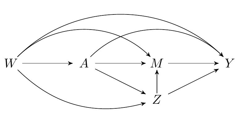
FIGURE 7.1: Directed acyclic graph under intermediate confounders of the mediator-outcome relation affected by treatment

Recall that the interventional (in)direct effects are defined via the decomposition: \[\begin{equation*} \E[Y_{1,G_1} - Y_{0,G_0}] = \underbrace{\E[Y_{\color{red}{1},\color{blue}{G_1}} - Y_{\color{red}{1},\color{blue}{G_0}}]}_{\text{interventional indirect effect}} + \underbrace{\E[Y_{\color{blue}{1},\color{red}{G_0}} - Y_{\color{blue}{0},\color{red}{G_0}}]}_{\text{interventional direct effect}} \end{equation*}\]

In our data example, we’ll consider the eating of snacks as a potential intermediate confounder, since one might reasonably hypothesize that participation on a sports team might subsequently affect snacking, which then could affect mediators like the amount of exercises and overweight status.
The interventional direct and indirect effects may also be easily estimated with the medoutcon R package (Hejazi, Dı́az, and Rudolph 2022; Hejazi, Rudolph, and Dı́az 2022).
Just as for the natural (in)direct effects, medoutcon implements cross-validated one-step and TML estimators of the interventional effects.

7.1.5 Efficient estimation of the interventional (in)direct effects

Estimation of these effects is more complex, so a few additional nuisance parameters arise when expressing the (more general) EIF for these effects:
- \(q(z \mid a, w)\), the conditional density of the intermediate confounders, conditional only on treatment and baseline covariates;
- \(r(z \mid a, m, w)\), the conditional density of the intermediate confounders, conditional on mediators, treatment, and baseline covariates.
To estimate the interventional effects, we only need to set the argument Z of medoutcon to a value other than NULL.
Note that the implementation in medoutcon is currently limited to settings with only binary intermediate confounders, i.e., \(Z \in \{0, 1\}\).
Let’s use medoutcon() to estimate the interventional direct effect:

# compute one-step estimate of the interventional direct effect
interv_de_onestep <- medoutcon(
  W = weight_behavior[, c("age", "sex", "race", "tvhours")],
  A = (as.numeric(weight_behavior$sports) - 1),
  Z = (as.numeric(weight_behavior$snack) - 1),
  M = weight_behavior[, c("exercises", "overweigh")],
  Y = weight_behavior$bmi,
  g_learners = lasso_lrnr,
  h_learners = lasso_lrnr,
  b_learners = lasso_lrnr,
  effect = "direct",
  estimator = "onestep",
  estimator_args = list(cv_folds = 5)
)
summary(interv_de_onestep)
#> # A tibble: 1 × 7
#>   lwr_ci param_est upr_ci var_est  eif_mean estimator param                
#>    <dbl>     <dbl>  <dbl>   <dbl>     <dbl> <chr>     <chr>                
#> 1 -0.344     0.231  0.806  0.0861 -1.66e-16 onestep   direct_interventional

We can similarly estimate the interventional indirect effect:

# compute one-step estimate of the interventional indirect effect
interv_ie_onestep <- medoutcon(
  W = weight_behavior[, c("age", "sex", "race", "tvhours")],
  A = (as.numeric(weight_behavior$sports) - 1),
  Z = (as.numeric(weight_behavior$snack) - 1),
  M = weight_behavior[, c("exercises", "overweigh")],
  Y = weight_behavior$bmi,
  g_learners = lasso_lrnr,
  h_learners = lasso_lrnr,
  b_learners = lasso_lrnr,
  effect = "indirect",
  estimator = "onestep",
  estimator_args = list(cv_folds = 5)
)
summary(interv_ie_onestep)
#> # A tibble: 1 × 7
#>   lwr_ci param_est upr_ci var_est eif_mean estimator param                  
#>    <dbl>     <dbl>  <dbl>   <dbl>    <dbl> <chr>     <chr>                  
#> 1  0.529      1.07   1.61  0.0765 2.04e-15 onestep   indirect_interventional

From the above, we can conclude that the effect of participation on a sports team on BMI is largely through the interventional indirect effect (i.e., through the pathways involving the mediating variables) rather than via its direct effect.
Just as before, we could have instead used the TML estimators, instead of the one-step estimators. Doing this is as simple as setting the estimator = "tmle" in the relevant argument.

7.2 `medshift`: Stochastic (in)direct effects

While the analyses using the natural and interventional effects have been illuminating, we may also go beyond the restrictive static interventions required to define these (in)direct effects. In fact, it may be more realistic to consider interventions that do not directly force children to join athletic teams, but instead motivate them to make their participation on such teams more likely. Importantly, such interventions are often far more realistic and actionable in real-world studies.

7.2.1 Formulating the stochastic (in)direct effects

These more flexible intervention regimes are incompatible with (in)direct effect definitions based on decomposing the average treatment effect.
Instead, consider the decomposition of the population intervention effect (PIE) of a stochastic intervention into direct and indirect effects (Dı́az and Hejazi 2020): \[\begin{align*} \E[Y&_{A_\delta,M_{A_\delta}} - Y_{A,M_A}] = \\ &\underbrace{\E[Y_{\color{red}{A_\delta},\color{blue}{M_{A_\delta}}} - Y_{\color{red}{A_\delta},\color{blue}{M}}]}_{\text{stochastic natural indirect effect}} + \underbrace{\E[Y_{\color{blue}{A_\delta},\color{red}{M}} - Y_{\color{blue}{A},\color{red}{M}}]}_{\text{stochastic natural direct effect}} \end{align*}\]
Recall from our discussion of the incremental propensity score interventions (Kennedy 2018) that such stochastic interventions can compare the pre- and post-intervention odds of exposure: \[\begin{equation*} \delta = \frac{\text{odds}(A_\delta = 1\mid W=w)} {\text{odds}(A = 1\mid W=w)}. \end{equation*}\]
In our analysis, we will modulate the odds of participating in a sports team by a fixed amount for each individual, setting, for example, \(\delta = 2\):

delta_shift_ipsi <- 2

Such an intervention may be interpreted as the effect of a school program that motivates children to participate in sports teams.

7.2.2 Efficient estimation of the stochastic (in)direct effects

The decomposition of the PIE into the direct and indirect effects leads to a common term \(\E[Y_{\color{red}{A_\delta},\color{blue}{M}}]\) involved in both the direct and indirect effect definitions. This term may be estimated via the medshift R package (Hejazi and Dı́az 2020).
For the direct effect, the remaining term is the \(\E[Y_{\color{blue}{A},\color{red}{M}}]\), which may be estimated by a simple mean in the observed data (i.e., no intervention).
For the indirect effect, the remaining term is the joint effect of stochastic interventions on both \(A\) and \(M\): \(\E[Y_{\color{red}{A_\delta},\color{blue}{M_{A_\delta}}}\).
- For the case of an IPSI on binary \(A\), this may be estimated by the tools in the npcausal R package.
- For the case of an MTP on continuous \(A\), this may be estimated by the tools in the txshift R package (Hejazi and Benkeser 2020a, 2020b).
Like the implementation in medoutcon, the medshift package makes use of cross-validation in constructing initial estimates of nuisance parameters, resulting in more robust, cross-validated efficient estimators (Klaassen 1987; Zheng and van der Laan 2011; Chernozhukov et al. 2018).
Now, we’re ready to use the medshift function to estimate the decomposition term common to both the stochastic direct and indirect effects:

# compute one-step estimate of the decomposition term of the (in)direct effects
stoch_decomp_onestep <- medshift(
  W = weight_behavior[, c("age", "sex", "race", "tvhours")],
  A = (as.numeric(weight_behavior$sports) - 1),
  Z = weight_behavior[, c("snack", "exercises", "overweigh")],
  Y = weight_behavior$bmi,
  delta = delta_shift_ipsi,
  g_learners = lasso_lrnr,
  e_learners = lasso_lrnr,
  m_learners = lasso_lrnr,
  estimator = "onestep",
  estimator_args = list(cv_folds = 5)
)
summary(stoch_decomp_onestep)
#>      lwr_ci   param_est      upr_ci   param_var    eif_mean   estimator 
#>   18.749473   19.081534   19.413595    0.028704 -1.1843e-15     onestep

To estimate the stochastic direct effect, an extra step is necessary – we must apply the delta method:

# convenience function to compute inference via delta method: EY1 - EY0
linear_contrast <- function(params, eifs, ci_level = 0.95) {
  # bounds for confidence interval
  ci_norm_bounds <- c(-1, 1) * abs(stats::qnorm(p = (1 - ci_level) / 2))
  param_est <- params[[1]] - params[[2]]
  eif <- eifs[[1]] - eifs[[2]]
  se_eif <- sqrt(var(eif) / length(eif))
  param_ci <- param_est + ci_norm_bounds * se_eif
  # parameter and inference
  out <- c(param_ci[1], param_est, param_ci[2])
  names(out) <- c("lwr_ci", "param_est", "upr_ci")
  return(out)
}

Straightforward application of this procedure yields,

# parameter estimates and EIFs for components of direct effect
EY <- mean(weight_behavior$bmi)
eif_EY <- weight_behavior$bmi - EY
params_de <- list(stoch_decomp_onestep$theta, EY)
eifs_de <- list(stoch_decomp_onestep$eif, eif_EY)

# direct effect = EY - estimated quantity
de_est <- linear_contrast(params_de, eifs_de)
de_est
#>    lwr_ci param_est    upr_ci 
#> -0.509201 -0.045574  0.418053

From the above, we can conclude that the effect of increasing the odds of participation on a sports team on BMI leads only to a relatively small direct effect.

Chapter 7 R packages for estimation of the causal (in)direct effects

7.1 medoutcon: Natural and interventional (in)direct effects