# Causal mediation analysis intro {#mediation}
```{r}
#| label: load-renv
#| echo: false
#| message: false
renv::autoload()
library(here)
```
## Motivating study
- We recently estimated the risk of opioid use disorder and opioid overdose
that is due to having a chronic pain condition or a physical disability (total
effects).
- Having a chronic pain condition (without disability) more than doubled the
risk (3.6% developed OUD in 18 mo).
- Having a physical disability (without chronic pain) increased risk by more
than 1.6 times (2.9% developed OUD).
- To what extent are these total risks explained by the pain management
treatments that result from these conditions? Which treatments are more risky?
Which are less risky?
- We can to use mediation analysis to explore the pain management mechanisms
contributing to these risks.
- Key questions:
- To what extent does the effect of having a disability or chronic pain
condition at the time of Medicaid enrollment on subsequent OUD risk operate
through pain management strategies? Considered as a bundle? And one-by-one?
[@rudolph2025mediation]
{width=120% fig-align="center"}
{width=120% fig-align="center"}
## What is causal mediation analysis?
- Statistical mediation analyses assess associations between the variables.
They can help you establish, for example, if the *association* between
treatment and outcome can be mostly explained by an *association* between
treatment and mediator
- Causal mediation analyses, on the other hand, seek to assess causal
relations. For example, they help you establish whether treatment *causes* the
outcome because it *causes* the mediator. To do this, causal mediation seek to
understand how the paths behave under circumstances different from the
observed circumstances (e.g., interventions)
<!--- Causal mediation analysis is thus useful to understand mechanisms-->
### Why are the causal methods that we will discuss today important?
- Assume you are interested in the effect of treatment assignment $A$ (e.g.,
chronic pain condition vs. neither chronic pain nor physical disability) on
an outcome $Y$ (risk of OUD) through mediators $M$ (e.g., opioid prescriptions,
co-prescriptions, anti-depressants and anti-inflammatories, physical therapy)
- We have pre-treatment confounders $W$
- When considering particular pain management treatments, there are
intermediate confounders, $Z$, of the $M \rightarrow Y$ relationship that are
affected by chronic pain: other co-occurring or upstream pain management
treatments
- We could fit the following models:
\begin{align}
\E(M \mid A=a, W=w, Z=z) & = \gamma_0 + \gamma_1 a + \gamma_2 w + \gamma_3 z \\
\E(Y \mid M=m, A=a, W=w, Z=z) & = \beta_0 + \beta_1 m + \beta_2 a + \beta_3 w + \beta_4 z
\end{align}
- The product $\gamma_1 \beta_1$ has been proposed as a measure of the effect
of $A$ on $Y$ through $M$
- Causal interpretation problems with this method: We will see that this
parameter cannot be interpreted as a causal effect
### `R` Example:
- Assume we have a pre-treatment confounder of $Y$ and $M$, denote it with $W$
- For simplicity, assume $A$ is randomized
- We'll generate a really large sample from a data generating mechanism so that
we are not concerned with sampling errors
```{webr-r}
n <- 1e6
w <- rnorm(n)
a <- rbinom(n, 1, 0.5)
z <- rbinom(n, 1, 0.2 * a + 0.3)
m <- rnorm(n, w + z)
y <- rnorm(n, m + w - a + z)
```
- Note that the indirect effect (i.e., the effect through $M$) in this example
is nonzero (there is a pathway $A \rightarrow Z \rightarrow M \rightarrow Y$)
- Let's see what the product of coefficients method would say:
```{webr-r}
lm_y <- lm(y ~ m + a + w + z)
lm_m <- lm(m ~ a + w + z)
## product of coefficients
coef(lm_y)[2] * coef(lm_m)[2]
```
Among other things, in this workshop:
- We will provide some understanding for why the above method fails in this
example
- We will study estimators that are robust to misspecification in the above
models
## Causal mediation models
In this workshop we will use directed acyclic graphs. We will focus on the two
types of graph:
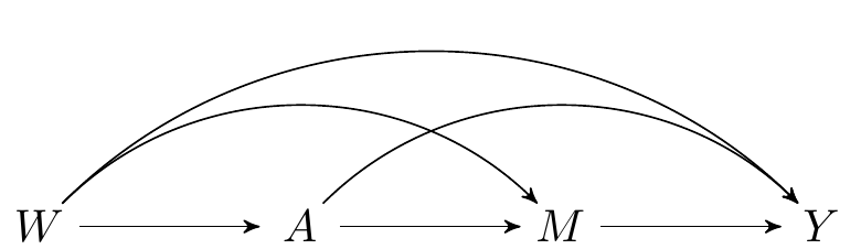
### No intermediate confounders
```{tikz}
%| fig-cap: Directed acyclic graph under *no intermediate confounders* of the mediator-outcome relation affected by treatment
\dimendef\prevdepth=0
\pgfdeclarelayer{background}
\pgfsetlayers{background,main}
\usetikzlibrary{arrows,positioning}
\tikzset{
>=stealth',
punkt/.style={
rectangle,
rounded corners,
draw=black, very thick,
text width=6.5em,
minimum height=2em,
text centered},
pil/.style={
->,
thick,
shorten <=2pt,
shorten >=2pt,}
}
\newcommand{\Vertex}[2]
{\node[minimum width=0.6cm,inner sep=0.05cm] (#2) at (#1) {$#2$};
}
\newcommand{\VertexR}[2]
{\node[rectangle, draw, minimum width=0.6cm,inner sep=0.05cm] (#2) at (#1) {$#2$};
}
\newcommand{\ArrowR}[3]
{ \begin{pgfonlayer}{background}
\draw[->,#3] (#1) to[bend right=30] (#2);
\end{pgfonlayer}
}
\newcommand{\ArrowL}[3]
{ \begin{pgfonlayer}{background}
\draw[->,#3] (#1) to[bend left=45] (#2);
\end{pgfonlayer}
}
\newcommand{\EdgeL}[3]
{ \begin{pgfonlayer}{background}
\draw[dashed,#3] (#1) to[bend right=-45] (#2);
\end{pgfonlayer}
}
\newcommand{\Arrow}[3]
{ \begin{pgfonlayer}{background}
\draw[->,#3] (#1) -- +(#2);
\end{pgfonlayer}
}
\begin{tikzpicture}
  \Vertex{-4, 0}{W}
  \Vertex{0, 0}{M}
  \Vertex{-2, 0}{A}
  \Vertex{2, 0}{Y}
  \Arrow{W}{A}{black}
  \Arrow{A}{M}{black}
  \Arrow{M}{Y}{black}
  \ArrowL{W}{Y}{black}
  \ArrowL{A}{Y}{black}
  \ArrowL{W}{M}{black}
\end{tikzpicture}
```
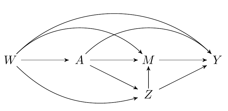
### Intermediate confounders
```{tikz}
%| fig-cap: Directed acyclic graph under intermediate confounders of the mediator-outcome relation affected by treatment
\dimendef\prevdepth=0
\pgfdeclarelayer{background}
\pgfsetlayers{background,main}
\usetikzlibrary{arrows,positioning}
\tikzset{
>=stealth',
punkt/.style={
rectangle,
rounded corners,
draw=black, very thick,
text width=6.5em,
minimum height=2em,
text centered},
pil/.style={
->,
thick,
shorten <=2pt,
shorten >=2pt,}
}
\newcommand{\Vertex}[2]
{\node[minimum width=0.6cm,inner sep=0.05cm] (#2) at (#1) {$#2$};
}
\newcommand{\VertexR}[2]
{\node[rectangle, draw, minimum width=0.6cm,inner sep=0.05cm] (#2) at (#1) {$#2$};
}
\newcommand{\ArrowR}[3]
{ \begin{pgfonlayer}{background}
\draw[->,#3] (#1) to[bend right=30] (#2);
\end{pgfonlayer}
}
\newcommand{\ArrowL}[3]
{ \begin{pgfonlayer}{background}
\draw[->,#3] (#1) to[bend left=45] (#2);
\end{pgfonlayer}
}
\newcommand{\EdgeL}[3]
{ \begin{pgfonlayer}{background}
\draw[dashed,#3] (#1) to[bend right=-45] (#2);
\end{pgfonlayer}
}
\newcommand{\Arrow}[3]
{ \begin{pgfonlayer}{background}
\draw[->,#3] (#1) -- +(#2);
\end{pgfonlayer}
}
\begin{tikzpicture}
  \Vertex{0, -1}{Z}
  \Vertex{-4, 0}{W}
  \Vertex{0, 0}{M}
  \Vertex{-2, 0}{A}
  \Vertex{2, 0}{Y}
  \ArrowR{W}{Z}{black}
  \Arrow{Z}{M}{black}
  \Arrow{W}{A}{black}
  \Arrow{A}{M}{black}
  \Arrow{M}{Y}{black}
  \Arrow{A}{Z}{black}
  \Arrow{Z}{Y}{black}
  \ArrowL{W}{Y}{black}
  \ArrowL{A}{Y}{black}
  \ArrowL{W}{M}{black}
\end{tikzpicture}
```
The above graphs can be interpreted as a *non-parametric structural equation
model* (NPSEM), also known as a *structural causal model* (SCM):
\begin{align}
W & = f_W(U_W) \nonumber \\
A & = f_A(W, U_A) \nonumber \\
Z & = f_Z(W, A, U_Z) \nonumber \\
M & = f_M(W, A, Z, U_M) \nonumber \\
Y & = f_Y(W, A, Z, M, U_Y)
\end{align}
- Here $U=(U_W, U_A, U_Z, U_M, U_Y)$ is a vector of all unmeasured exogenous
factors affecting the system
- The functions $f$ are assumed fixed but unknown
- We posit this model as a system of equations that nature uses to generate the
data
- Therefore we leave the functions $f$ unspecified (i.e., we do not know the
true nature mechanisms)
- Sometimes we know something: e.g., if $A$ is randomized we know $A=f_A(U_A)$
where $U_A$ is the flip of a coin (i.e., independent of everything).
## Counterfactuals
- Recall that we are interested in assessing how the pathways would behave
under circumstances different from the observed circumstances
- We operationalize this idea using *counterfactual* random variables
- Counterfactuals are hypothetical random variables that would have been
observed in an alternative world where something had happened, possibly
contrary to fact
<!--we would be able to perform interventions on the random variables of interest-->
### We will use the following counterfactual variables:
- $Y_a$ is a counterfactual variable in a hypothetical world where $\P(A=a)=1$
for some value $a$
- $Y_{a,m}$ is the counterfactual outcome in a world where $\P(A=a,M=m)=1$
- $M_a$ is the counterfactual variable representing the mediator in a world
where $\P(A=a)=1$.
### How are counterfactuals defined?
<!-- - You can use counterfactual variables as _primitives_ -->
- In the NPSEM framework, counterfactuals are quantities *derived* from the
model.
- Once you define a change to the causal system, that change needs to be
propagated downstream.
- Example: modifying the system to make everyone receive XR-NTX yields
counterfactual adherence, mediators, and outcomes.
- Take as example the DAG in Figure 1.2:
\begin{align}
A &= a \nonumber \\
Z_a &= f_Z(W, a, U_Z) \nonumber \\
M_a &= f_M(W, a, Z_a, U_M) \nonumber \\
Y_a &= f_Y(W, a, Z_a, M_a, U_Y)
\end{align}
- We will also be interested in *joint changes* to the system:
\begin{align}
A &= a \nonumber \\
Z_a &= f_Z(W, a, U_Z) \nonumber \\
M &= m \nonumber \\
Y_{a, m} &= f_Y(W, a, Z_a, m, U_Y)
\end{align}
- And, perhaps more importantly, we will use *nested counterfactuals*
- For example, if $A$ is binary, you can think of the following counterfactual
\begin{align}
A &= 1 \nonumber \\
Z_1 &= f_Z(W, 1, U_Z) \nonumber \\
M &= M_0 \nonumber \\
Y_{1, M_0} &= f_Y(W, 1, Z_1, M_0, U_Y)
\end{align}
- $Y_{1, M_0}$ is interpreted as *the outcome for an individual in a
hypothetical world where treatment was given, but the mediator was held at
the value it would have taken under no treatment*.
- Causal mediation effects are often defined in terms of the distribution of
these nested counterfactuals.
- That is, causal effects give you information about what would have happened
*in some hypothetical world* where the mediator and treatment mechanisms
changed.