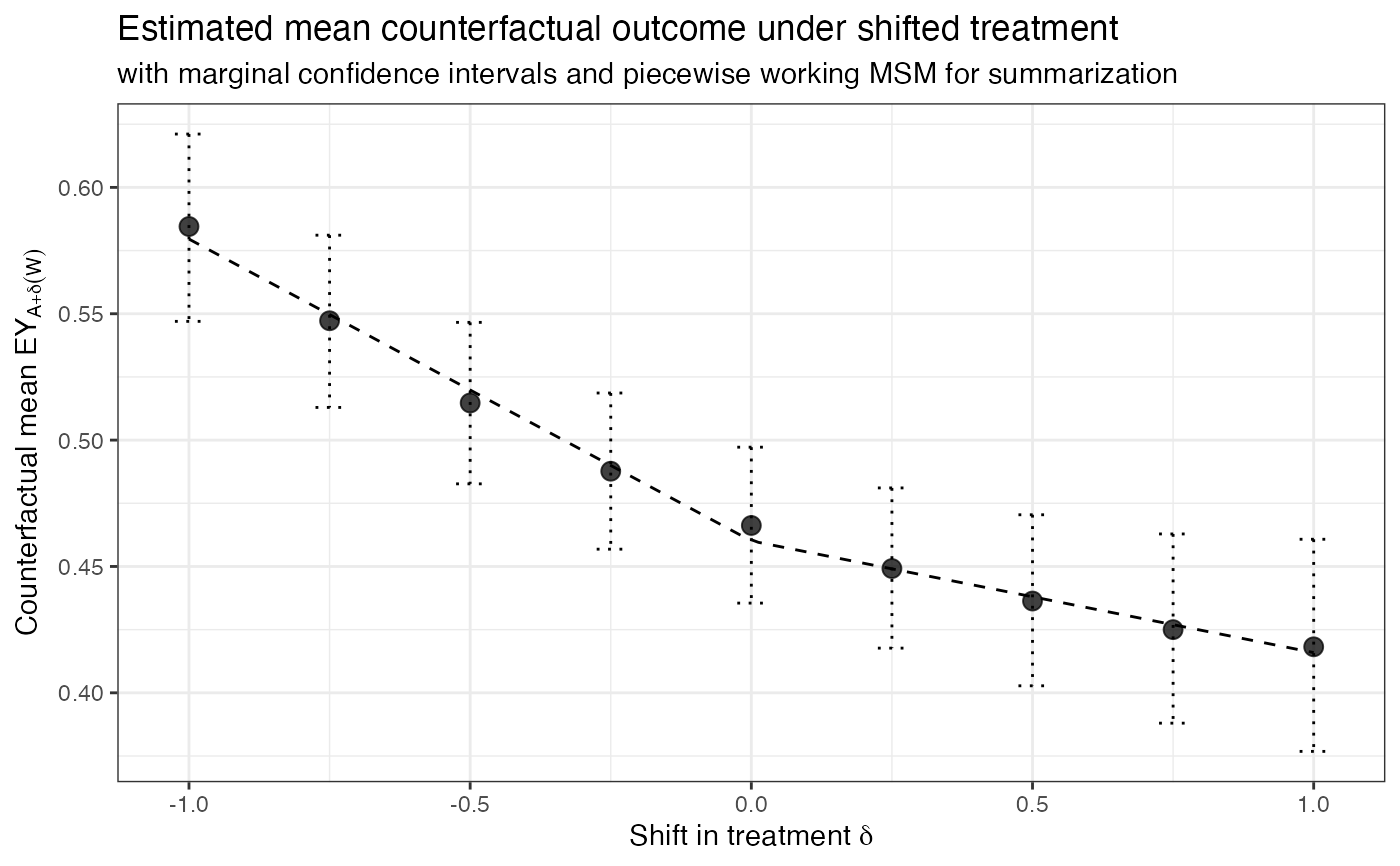
Plot working MSM for causal effects of an intervention grid

# S3 method for class 'txshift_msm'
plot(x, ...)

Arguments

x: Object of class txshift_msm as produced by a call to msm_vimshift.
...: Additional arguments passed to plot as necessary.

Details

Creates a visualization of the intervention-specific counterfactual means as well as the working marginal structural model summarizing the trend across posited values of the intervention.

Examples

if (require("sl3")) {
  set.seed(3287)
  n_obs <- 1000
  W <- as.numeric(replicate(1, rbinom(n_obs, 1, 0.5)))
  A <- as.numeric(rnorm(n_obs, mean = 2 * W, sd = 1))
  Y <- rbinom(n_obs, 1, plogis(2 * A - W))
  msm <- msm_vimshift(
    W = W, A = A, Y = Y, estimator = "tmle",
    g_exp_fit_args = list(
      fit_type = "sl",
      sl_learners_density = Lrnr_density_hse$new(Lrnr_glm$new())
    ),
    Q_fit_args = list(
      fit_type = "glm",
      glm_formula = "Y ~ ."
    ),
    delta_grid = seq(-1, 1, 0.25)
  )
  plot(msm)

  # fit a linear spline with knot at 0
  set.seed(8293)
  n_obs <- 1000
  W <- as.numeric(replicate(1, rbinom(n_obs, 1, 0.5)))
  A <- as.numeric(rnorm(n_obs, mean = 2 * W, sd = 1))
  Y <- rbinom(n_obs, 1, plogis(0.1 * A * (A >= 0) - 3 * A * (A < 0) - W))
  msm <- msm_vimshift(
    W = W, A = A, Y = Y, estimator = "tmle",
    g_exp_fit_args = list(
      fit_type = "sl",
      sl_learners_density = Lrnr_density_hse$new(Lrnr_glm$new())
    ),
    Q_fit_args = list(
      fit_type = "glm",
      glm_formula = "Y ~ ."
    ),
    delta_grid = seq(-1, 1, 0.25),
    msm_form = list(type = "piecewise", knot = 0)
  )
  plot(msm)
}