Highly Adaptive Lasso Conditional Density Estimation

Background and motivation

In causal inference problems, both classical estimators (e.g., inverse probability weighting) and doubly robust estimators (e.g., one-step estimation, targeted minimum loss estimation) require estimation of the propensity score, a nuisance parameter corresponding to the treatment mechanism. While treatments of interest may often be continuous-valued, most approaches opt to discretize the treatment so as to estimate effects based on binary (or categorical) treatment. Such simplifications are often motivated by convenience rather than science – to avoid estimation of the generalized propensity score (Hirano and Imbens 2004; Imai and Van Dyk 2004), the covariate-conditional treatment density. The haldensify package introduces a flexible approach for estimating such conditional density functions, using the highly adaptive lasso (HAL), a nonparametric estimator that has been shown to exhibit desirable rate-convergence properties.

Consider data generated by typical cohort sampling $O = (W, A, Y)$ , where $W$ is a vector of baseline covariates, $A$ is a continuous (or ordinal) treatment, and $Y$ is an outcome of interest. Estimation of the generalized propensity score $g_{0,A}$ corresponds to estimating the conditional density of $A$ given $W = w$ . A simple strategy for estimating this nuisance function is to assume a parametric working model and use parametric regression to generate suitable density estimates. For example, one could operate under the working assumption that $A$ given $W$ follows a Gaussian distribution with homoscedastic variance and mean $\sum_{j=1}^p \beta_j \phi_j(W)$ , where $\phi = (\phi_j : j)$ are user-selected basis functions and $\beta = (\beta_j : j)$ are unknown regression parameters. In this case, a density estimate would be generated by fitting a linear regression of $A$ on $\phi(W)$ to estimate the conditional mean of $A$ given $W$ , paired with maximum likelihood estimation of the variance of $A$ . Then, the estimated conditional density would be given by the density of a Gaussian distribution evaluated at these estimates. Unfortunately, most such approaches do not allow for flexible modeling of $g_{0,A}$ . This motivated our development of a novel and flexible procedure for constructing conditional density estimators $g_{n,A}(a \mid w)$ of $A$ given $W = w$ (possibly subject to observation-level weights).

Conditional density estimation by pooled hazards regression

As consistent estimation of the generalized propensity score is an integral part of constructing estimators of the causal effects of continuous treatments, our conditional density estimator, built around the HAL regression function, may be quite useful in flexibly constructing such estimates. We note that proposals for the data adaptive estimation of such quantities are sparse in the literature (e.g., Zhu, Coffman, and Ghosh (2015)). Notably, Dı́az and van der Laan (2011) gave a proposal for constructing a semiparametric estimator of such a target quantity based on exploiting the relationship between the hazard and density functions. Our proposal builds upon theirs in several key ways:

we adjust their algorithm so as to incorporate sample-level weights, necessary for making use of sample-level weights (e.g., inverse probability of censoring weighting); and
we replace their use of an arbitrary classification model with the HAL regression function.

While our first modification is general and may be applied to the estimation strategy of Dı́az and van der Laan (2011), our latter contribution requires adjusting the penalization aspect of HAL regression so as to respect the use of a loss function appropriate for density estimation on the hazard scale.

To build an estimator of a conditional density, Dı́az and van der Laan (2011) considered discretizing the observed $a \in A$ based on a number of bins $T$ and a binning procedure (e.g., including the same number of points in each bin or forcing bins to be of the same length). We note that the choice of the tuning parameter $T$ corresponds roughly to the choice of bandwidth in classical kernel density estimation; this will be made clear upon further examination of the proposed algorithm. The data $\{A, W\}$ are reformatted such that the hazard of an observed value $a \in A$ falling in a given bin may be evaluated via standard classification techniques. In fact, this proposal may be viewed as a re-formulation of the classification problem into a corresponding set of hazard regressions: $\begin{align*} \mathbb{P} (a \in [\alpha_{t-1}, \alpha_t) \mid W) =& \mathbb{P} (a \in [\alpha_{t-1}, \alpha_t) \mid A \geq \alpha_{t-1}, W) \times \\ & \prod_{j = 1}^{t -1} \{1 - \mathbb{P} (a \in [\alpha_{j-1}, \alpha_j) \mid A \geq \alpha_{j-1}, W) \}, \end{align*}$ where the probability that a value of $a \in A$ falls in a bin $[\alpha_{t-1}, \alpha_t)$ may be directly estimated from a standard classification model. The likelihood of this model may be re-expressed in terms of the likelihood of a binary variable in a data set expressed through a repeated measures structure. Specifically, this re-formatting procedure is carried out by creating a data set in which any given observation $A_i$ appears (repeatedly) for as many intervals $[\alpha_{t-1}, \alpha_t)$ that there are prior to the interval to which the observed $a$ belongs. A new binary outcome variable, indicating $A_i \in [\alpha_{t-1}, \alpha_t)$ , is recorded as part of this new data structure. With the re-formatted data, a pooled hazard regression, spanning the support of $A$ is then executed. Finally, the conditional density estimator $\begin{equation*} g_{n, \alpha}(a \mid W) = \frac{\mathbb{P}(a \in [\alpha_{t-1}, \alpha_t) \mid W)}{(\alpha_t - \alpha_{t-1})}, \end{equation*}$ for $\alpha_{t-1} \leq a \le \alpha_t$ , may be constructed. As part of this procedure, the hazard estimates are mapped to density estimates through rescaling of the estimates by the bin size ( $\alpha_t - \alpha_{t-1}$ ).

In its original proposal, a key element of this procedure was the use of any arbitrary classification procedure for estimating $\mathbb{P}(a \in [\alpha_{t-1}, \alpha_t) \mid W)$ , facilitating the incorporation of flexible, data adaptive estimators. We alter this proposal in two ways,

replacing the arbitrary estimator of $\mathbb{P}(a \in [\alpha_{t-1}, \alpha_t) \mid W)$ with HAL regression, and
accommodating the use of sample-level weights, making it possible for the resultant conditional density estimator to achieve a convergence rate with respect to a loss-based dissimilarity of $\approx n^{-1/3}$ under assumptions.

Our procedure alters the HAL regression function to use a loss function tailored for estimation of the hazard, invoking $\ell_1$ -penalization in a manner consistent with this loss.

Example: Conditional density estimation

First, let’s load a few required packages and set a seed for our example.

library(haldensify)
library(data.table)
library(ggplot2)
set.seed(75681)

Next, we’ll generate a simple simulated dataset. The function make_example_data, defined below, generates a baseline covariate $W$ and a continuous treatment $A$ , whose mean is a function of $W$ .

make_example_data <- function(n_obs) {
  W <- runif(n_obs, -4, 4)
  A <- rnorm(n_obs, mean = W, sd = 0.25)
  dat <- as.data.table(list(A = A, W = W))
  return(dat)
}

Now, let’s simulate our data and take a quick look at it:

# number of observations in our simulated dataset
n_obs <- 200
(example_data <- make_example_data(n_obs))

##               A           W
##           <num>       <num>
##   1:  2.3063922  2.24687273
##   2:  0.9297479  0.91025531
##   3: -3.2443382 -2.98696024
##   4: -0.1842217 -0.01204378
##   5:  3.2756387  3.59166824
##  ---                       
## 196:  0.4250425  0.43070281
## 197:  1.0606211  1.35836156
## 198:  2.2820014  2.34814939
## 199: -2.9015290 -3.05240270
## 200: -3.2334017 -3.52716556

Next, we’ll fit our pooled hazards conditional density estimator via the haldensify wrapper function. Based on underlying theory and simulation experiments, we recommend setting a relatively large number of bins and using a binning strategy that accommodates creating such a large number of bins.

haldensify_fit <- haldensify(
  A = example_data$A,
  W = example_data$W,
  n_bins = c(4, 6, 8),
  grid_type = "equal_range",
  lambda_seq = exp(seq(-0.1, -10, length = 300)),
  # the following are passed to hal9001::fit_hal() internally
  max_degree = 1,
  reduce_basis = 1 / sqrt(n_obs)
)

Having constructed the conditional density estimator, we can examine the empirical risk over the grid of choices of the $L_1$ regularization parameter $\lambda$ . To do this, we can simply call the available plot method, which uses the cross-validated conditional density fits in the cv_tuning_results slot of the haldensify object. For example,

p_risk <- plot(haldensify_fit)
p_risk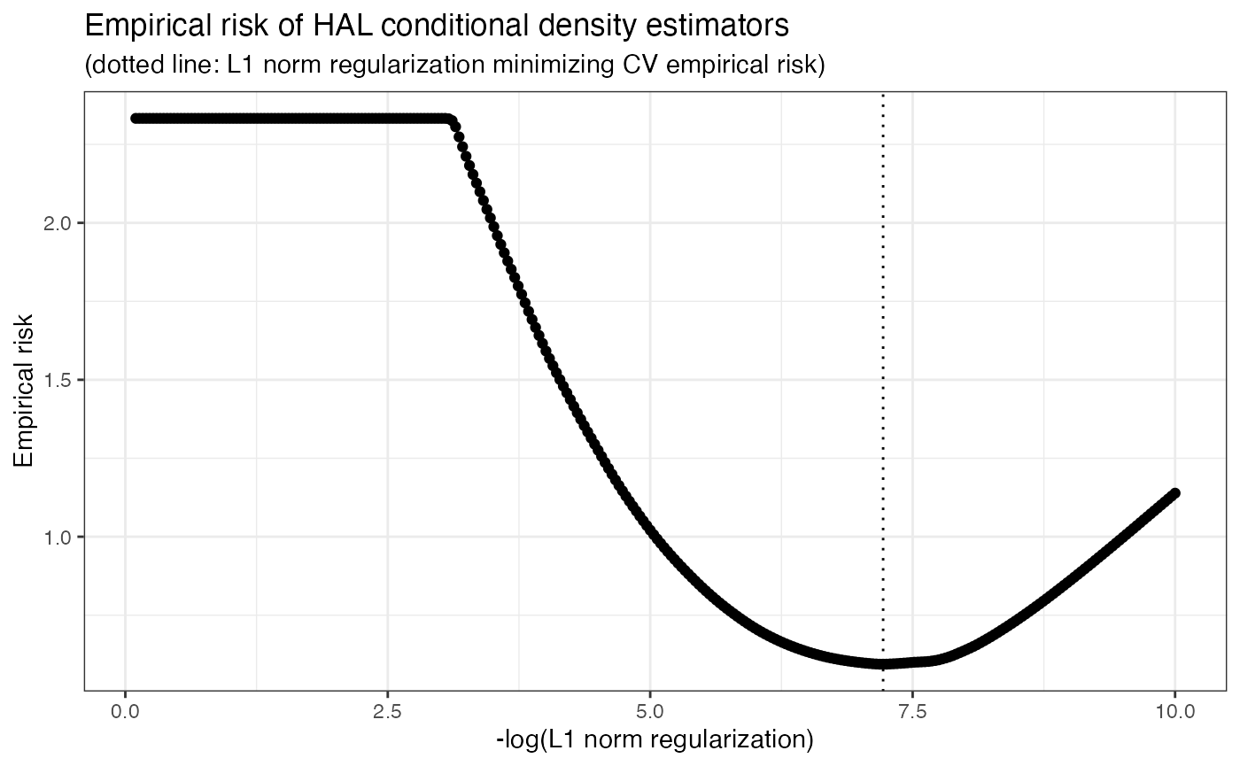

CV-risk of regularized conditional density estimators

Finally, we can predict the conditional density over the grid of observed values $A$ across different elements of the support $W$ . We do this using the predict method of haldensify and plot the results below.

# predictions to recover conditional density of A|W
new_a <- seq(-4, 4, by = 0.05)
new_dat <- as.data.table(list(
  a = new_a,
  w_neg = rep(-2, length(new_a)),
  w_zero = rep(0, length(new_a)),
  w_pos = rep(2, length(new_a))
))
new_dat[, pred_w_neg := predict(haldensify_fit,
  new_A = new_dat$a,
  new_W = new_dat$w_neg
)]
new_dat[, pred_w_zero := predict(haldensify_fit,
  new_A = new_dat$a,
  new_W = new_dat$w_zero
)]
new_dat[, pred_w_pos := predict(haldensify_fit,
  new_A = new_dat$a,
  new_W = new_dat$w_pos
)]
# visualize results
dens_dat <- melt(new_dat,
  id = c("a"),
  measure.vars = c("pred_w_pos", "pred_w_zero", "pred_w_neg")
)
p_dens <- ggplot(dens_dat, aes(x = a, y = value, colour = variable)) +
  geom_point() +
  geom_line() +
  stat_function(
    fun = dnorm, args = list(mean = -2, sd = 0.25),
    colour = "blue", linetype = "dashed"
  ) +
  stat_function(
    fun = dnorm, args = list(mean = 0, sd = 0.25),
    colour = "darkgreen", linetype = "dashed"
  ) +
  stat_function(
    fun = dnorm, args = list(mean = 2, sd = 0.25),
    colour = "red", linetype = "dashed"
  ) +
  labs(
    x = "Observed value of W",
    y = "Estimated conditional density",
    title = "Conditional density estimates g(A|W)"
  ) +
  theme_bw() +
  theme(legend.position = "none")
p_dens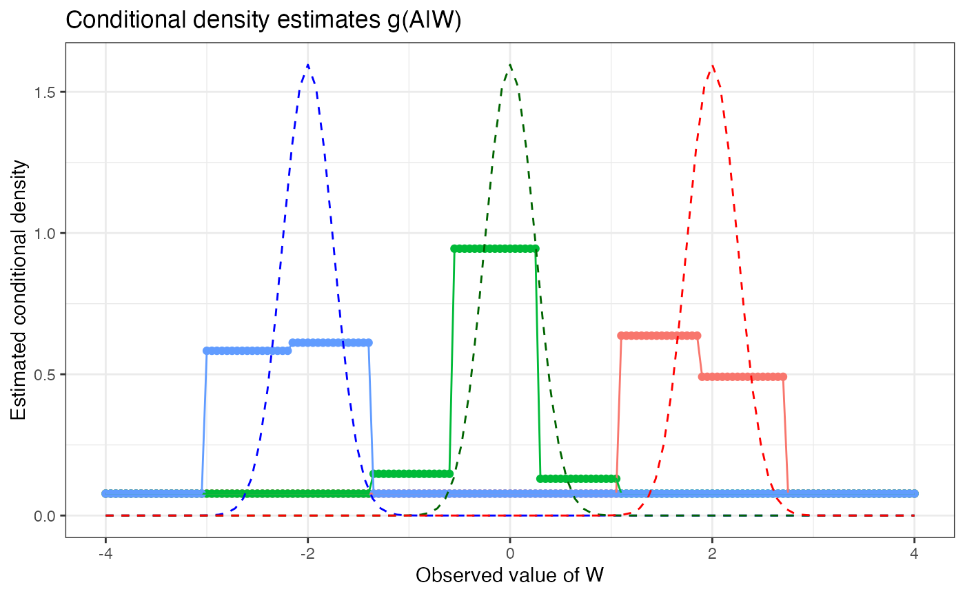

Estimated conditional density of A|W for several choices of W

In the above example, we generate synthetic data along a grid of $A$ and three values of $W$ ( $W \in \{-2, 0, +2\}$ ), representing distinct groups/strata with respect to the covariate $W$ . Using this data, we use the trained haldensify model to predict the density of $A$ , conditional on the paired value of $W$ , yielding estimates of the conditional density for each of these three hypothetical strata of $W$ . The resultant figure depicts the estimated conditional density as colored points (blue for $W = -2$ , green for $W = 0$ , and red for $W = +2$ ), and the theoretical density for each group as smooth curves (using ggplot2’s stat_function()). For each group, the differences between the estimated conditional densities and the theoretical densities can be taken as indicative of the quality of the haldensify estimator in this example. Overall, the haldensify estimator appears to recover the underlying density of $A$ best for the group $W = 0$ , with slightly degraded performance for $W = -2$ , which degrades further for $W = +2$ . The haldensify conditional density estimator has been used to estimate the generalized propensity score in applications of the methodology described in Hejazi et al. (2020).

Nonparametric inverse probability weighted estimation

As mentioned above, the generalized propensity score is a critical ingredient in evaluating causal effects for continuous treatments. A popular framework for defining and evaluating such causal effects is that of modified treatment policies (Haneuse and Rotnitzky 2013; Dı́az and van der Laan 2018; Hejazi et al. 2022), which define interventions that shift (or modify) the treatment. For example, in a setting with a continuous treatment $A$ , in which we additionally collect baseline covariates $W$ and an outcome measurement $Y$ (so that the data on a given unit is $O = (W, A, Y)$ ), we could consider an intervention that sets the value of $A$ via $d(A,W; \delta) = A + \delta(W)$ , for a user-defined function $d(A,W;\delta)$ indexed by a function (or scalar) $\delta$ . This intervention regime is a simple example of a modified treatment policy (MTP); it can be thought of mapping the observed $A$ to a counterfactual $A_{\delta}$ that is itself an additive shift of the natural value of $A$ . The counterfactual mean of such an intervention would be expressed $\mathbb{E}[Y(A_{\delta})]$ , where $Y(A_{\delta})$ is the potential outcome that would be observed had the treatment taken the value $A_{\delta}$ . Both Haneuse and Rotnitzky (2013) and Dı́az and van der Laan (2018) proposed substitution, inverse probability weighted (IPW), and doubly robust estimators of a statistical functional $\psi$ that identifies this counterfactual mean under standard assumptions. Doubly robust estimators of $\psi$ are implemented in the txshift R package (Hejazi and Benkeser 2020, 2022); such estimation frameworks are usually necessary in order to take advantage of flexible estimators of nuisance parameters.

Despite the popularity of doubly robust estimation procedures, IPW estimators can be modified to accommodate data adaptive estimation of the (generalized) propensity score. Such nonparametric IPW estimators, based on HAL, have been described by Ertefaie, Hejazi, and van der Laan (2022) in the context of binary treatments, and by Hejazi et al. (2022) for continuous treatments. The IPW estimator of $\psi$ is $\psi_{n,\text{IPW}} = \{\tilde{g}_{n,A}(A \mid W) / g_{n,A}(A \mid W)\} Y$ , where $g_{n,A}$ is an estimator of the generalized propensity score (e.g., as produced by haldensify()) and $\tilde{g}_{n,A}$ is this quantity evaluated at the post-intervention value of the treatment $A_{\delta}$ . Usually, $g_{n,A}$ must be estimated via parametric modeling strategies in order for $\psi_{n,\text{IPW}}$ to achieve desirable asymptotic properties (unbiasedness, efficiency); however, when $g_{n,A}$ is estimated flexibly, sieve estimation strategies (undersmoothing) may be used to select an estimator $g_{n,A}$ , from among an appropriate class, that allows for optimal estimation of $\psi$ . This issue arises in part because strategies for optimal selection of $g_{n,A}$ (e.g., cross-validation) optimize for estimation of the conditional density, ignoring the fact that it is only a nuisance parameter in the process of IPW estimation. When haldensify() is used for this purpose, a family of conditional density estimators $g_{n,A,\lambda}$ , indexed by the $\ell_1$ regularization term $\lambda$ , are generated, with cross-validation used to select an optimal estimator from among this trajectory in $\lambda$ . We saw this above when we visualized the empirical risk profile of $g_{n,A}$ . While empirical risk minimization based on the framework of cross-validated loss-based estimation is appropriate for optimally estimating the generalized propensity score, the selected estimator will fail to yield an IPW estimator with desirable asymptotic properties; undersmoothing must be used to select a more appropriate estimator. The haldensify package implements nonparametric IPW estimators that incorporate undersmoothing in the ipw_shift() function, the use of which we demonstrate below.

Example: Nonparametric IPW estimation

To begin, we set up a new data-generating process and simulate data for $n = 200$ units from it. We will aim to estimate the counterfactual mean of $Y$ under an MTP that shifts $A$ by $\delta = 2$ .

# set up data-generating process
make_example_data <- function(n_obs) {
  W <- runif(n_obs, 1, 4)
  A <- rpois(n_obs, 2 * W + 1)
  Y <- rbinom(n_obs, 1, plogis(2 - A + W + 3))
  dat <- as.data.table(list(Y = Y, A = A, W = W))
  return(dat)
}

# generate data and take a look
(dat_obs <- make_example_data(n_obs = 200))

##          Y     A        W
##      <int> <int>    <num>
##   1:     0    11 2.817789
##   2:     1     7 3.086448
##   3:     1     2 1.411537
##   4:     1     6 2.913294
##   5:     1     5 3.374974
##  ---                     
## 196:     1     2 1.347253
## 197:     1     3 1.383259
## 198:     1     2 1.103883
## 199:     1     3 1.660835
## 200:     1     5 2.183518

With this dataset, we can now simply call the ipw_shift() function, providing arguments that specify the causal effect of interest (delta = 2) and tuning parameters for estimating the generalized propensity score (lambda_seq, cv_folds, n_bins). The selector_type argument specifies the type of undersmoothing to be used to select an appropriate IPW estimator (from among a sequence in $\lambda$ ); setting the option selector_type = "all" simply returns IPW estimators for each of the selectors implemented. For a formal description of the selectors and numerical experiments examining their performance, see Hejazi et al. (2022).

est_ipw <- ipw_shift(
  W = dat_obs$W, A = dat_obs$A, Y = dat_obs$Y,
  delta = 2,
  cv_folds = 5L,
  n_bins = 4L,
  bin_type = "equal_range",
  selector_type = "all",
  lambda_seq = exp(seq(-1, -10, length = 500L)),
  # arguments passed to hal9001::fit_hal()
  max_degree = 1,
  reduce_basis = 1 / sqrt(n_obs)
)
confint(est_ipw)

## # A tibble: 6 × 8
##   lwr_ci   psi upr_ci se_est type           l1_norm lambda_idx gn_nbins
##    <dbl> <dbl>  <dbl>  <dbl> <chr>            <dbl>      <dbl>    <int>
## 1  0.570 0.668  0.753 0.0469 gcv               10.3        254        4
## 2  0.570 0.668  0.753 0.0469 dcar_tol          10.3        254        4
## 3  0.561 0.657  0.741 0.0464 dcar_min          23.7        295        4
## 4  0.564 0.658  0.740 0.0452 lepski_plateau    30.7        301        4
## 5  0.561 0.657  0.741 0.0464 smooth_plateau    23.7        295        4
## 6  0.561 0.657  0.741 0.0464 hybrid_plateau    23.7        295        4

The confint() method used above simply creates confidence intervals (95%, by default) for each of the IPW estimates returned. Examining the output, we can see that the IPW estimator based on cross-validation ("gcv") differs from that based on minimization of an important criterion from semiparametric efficiency theory ("dcar_min"). These estimators have different asymptotic properties, with the latter guaranteed to solve an estimating function required for the characterization of asymptotically efficient estimators.

References

Dı́az, Iván, and Mark J van der Laan. 2011. “Super Learner Based Conditional Density Estimation with Application to Marginal Structural Models.” International Journal of Biostatistics 7 (1): 1–20. https://doi.org/10.2202/1557-4679.1356.

———. 2018. “Stochastic Treatment Regimes.” In Targeted Learning in Data Science: Causal Inference for Complex Longitudinal Studies, 167–80. Springer. https://doi.org/10.1007/978-3-319-65304-4_14.

Ertefaie, Ashkan, Nima S Hejazi, and Mark J van der Laan. 2022. “Nonparametric Inverse-Probability-Weighted Estimators Based on the Highly Adaptive Lasso.” Biometrics (in press). https://doi.org/10.1111/biom.13719.

Haneuse, Sebastian, and A Rotnitzky. 2013. “Estimation of the Effect of Interventions That Modify the Received Treatment.” Statistics in Medicine 32 (30): 5260–77. https://doi.org/10.1002/sim.5907.

Hejazi, Nima S, and David C Benkeser. 2020. “txshift: Efficient Estimation of the Causal Effects of Stochastic Interventions in R.” Journal of Open Source Software 5 (54): 2447. https://doi.org/10.21105/joss.02447.

———. 2022. txshift: Efficient Estimation of the Causal Effects of Stochastic Interventions. https://doi.org/10.5281/zenodo.4070042.

Hejazi, Nima S, David Benkeser, Iván Dı́az, and Mark J van der Laan. 2022. “Efficient Estimation of Modified Treatment Policy Effects Based on the Generalized Propensity Score.” arXiv. https://arxiv.org/abs/2205.05777.

Hejazi, Nima S, Mark J van der Laan, Holly E Janes, Peter B Gilbert, and David C Benkeser. 2020. “Efficient Nonparametric Inference on the Effects of Stochastic Interventions Under Two-Phase Sampling, with Applications to Vaccine Efficacy Trials.” Biometrics 77 (4): 1241–53. https://doi.org/10.1111/biom.13375.

Hirano, Keisuke, and Guido W Imbens. 2004. “The Propensity Score with Continuous Treatments.” Applied Bayesian Modeling and Causal Inference from Incomplete-Data Perspectives 226164: 73–84.

Imai, Kosuke, and David A Van Dyk. 2004. “Causal Inference with General Treatment Regimes: Generalizing the Propensity Score.” Journal of the American Statistical Association 99 (467): 854–66.

Zhu, Yeying, Donna L Coffman, and Debashis Ghosh. 2015. “A Boosting Algorithm for Estimating Generalized Propensity Scores with Continuous Treatments.” Journal of Causal Inference 3 (1): 25–40. https://doi.org/10.1515/jci-2014-0022.